Spacetime and 4-vectors - Classical Mechanics & Special Relativity for Starters

4.1Space time¶

In 3D space we define a point/coordinate by its components $(x,y,z)$ where all components have the same unit. We can do this also in 4D space time by an event $(ct,x,y,z)$ as $ct$ has unit length (it should be called time space by this ordering, but what ever). The same unit for all components is needed if we want to do geometry with the coordinates.

If we want to measure distances $\Delta s$ between two points $(x_1,y_1,z_1)$ and $(x_2,y_2,z_2)$ we do this in 3D Euclidean space as $\Delta s^2 = (x_2-x_1)^2+(y_2-y_1)^2+(z_2-z_1)^2 = \Delta x^2 + \Delta y^2 + \Delta z^2$ . These distances are Galileo invariant, observer $S$ and $S'$ moving with $\vec{V}$ measure the same distance $\Delta s^2 = \Delta s^{'2}$ . Note, that we take these two pints at the sam time $t$ : $t_1=t_2$ . Or rephrased: we perform the measurement in the rest frame of the object we measure. That makes sense: measuring the length of an object that is moving requires that we measure the left and right side at the same time. Otherwise, the motion of the object will interfere with our measurements of the length.

The above statement is easily shown by invoking the Galilei Transformation:

\begin{split} x' &= x - V t \\ y' &= y \\ z' &= z \\ t' &= t \end{split}

(1)

We transform the two points $(x_1,y_1,z_1)$ and $(x_2,y_2,z_2)$ at the same time $t$ , we get:

\begin{split} x'_1 &= x_1 - V t, x'_2 = x_2 - V t \Rightarrow x'_2 - x'_1 = x_2 - x_1\\ y'_1 &= y_1, y'_2 = y_2 \Rightarrow y'_2 - y'_1 = y_2 - y_1\\ z'_1 &= z_1, z'_2 = z_2 \Rightarrow z'_2 - z'_1 = z_2 - z_1\\ t' &= t \end{split}

(2)

If we want to measure distances in space time and require that the distance is now Lorentz invariant, we cannot measure distance the same way! If we measure in $S$ the positions at the same time, that will in general be at different times according to $S'$ . Time is relative!

To do geometry, measure angles etc. we need an inner product and the inner product provides a distance measure (a metric) by the norm. For 3D you know that for two vectors $\vec{r}_1$ and $\vec{r}_2$ : $\Delta s^2 = || \vec{r}_1-\vec{r}_2 || ^2 = (\vec{r}_1-\vec{r}_2)\cdot (\vec{r}_1-\vec{r}_2)= \Delta x^2 + \Delta y^2 + \Delta z^2$ . Clearly the inner product in 4D space time cannot be defined in the same way.

We want that two relativistic observers measure the same distance (e.g. between two events), that is, it must be Lorentz invariant. We start by noting that the speed of light is constant for both observers. A light wave traveling in $S$ and $S'$ must therefore obey

c^2t^2-x^2-y^2-z^2 = 0 = c^2t^{'2}-x^{'2}-y^{'2}-z^{'2}

(3)

Given this observation it is needed (and natural) to define the distance in space time as

d s^2 = c^2d t^2 - d x^2 - d y^2 - d z^2

(4)

!!! important “Warning” Notice directly that the distance $\Delta s^2$ can be negative! (And we are OK with that).

It is straightforward to show that the above distance $ds^2$ is indeed a Lorentz Invariant, i.e. $ds'^2 = ds^2$ . Suppose we have two events: $E_1: (ct,x,y,z)$ and $E_2: (c(t+dt),x+dx,y+dy,z+dz)$ . We can transform these to $S'$ via the standard Lorentz Transformation:

\begin{array}{rcl} ct'_2 &=& \gamma \left ( c(t+dt) - \frac{V}{c}(x+dx) \right ) \Rightarrow &cdt' &=& \gamma \left ( cdt - \frac{V}{c}dx \right ) \\ x'_2 &=& \gamma \left ( (x+dx) - \frac{V}{c}c(t+dt) \right ) \Rightarrow &cdx' &=& \gamma \left ( dx - \frac{V}{c}cdt \right ) \\ y'_2 &=& y_2 \Rightarrow &dy' &=& dy\\ z'_2 &=& z_2 \Rightarrow &dz' &=& dz \end{array}

(5)

Clearly, we do only have to concentrate on the $cdt$ and $dx$ terms:

\begin{array}{rcl} cdt'^2 - dx'^2 &=& \gamma^2 \left ( cdt - \frac{V}{c}dx\right )^2 - \gamma^2 \left ( dx - \frac{V}{c}cdt \right )^2 \\ &=& \gamma^2 \left ( c^2 dt^2 - 2 \frac{V}{c} cdtdx + \frac{V^2}{c^2}dx^2 - dx^2 + 2 \frac{V}{c} dxcdt - \frac{V^2}{c^2}c^2dt^2\right ) \\ &=& \underbrace{\gamma^2 \left ( 1 - \frac{V^2}{c^2} \right )}_{=1} \left ( c^2dt^2 - dx^2 \right) \\ &=& c^2dt^2 - dx^2 \\ \end{array}

(6)

Note that if we had used a + sign, that is $ds^2 \equiv c^2dt^2 + dx^2$ , we would not have arrived at a Lorentz Invariant.

Pythagoras gets mixed up

We are used to all kind of ‘obvious’ results that hold in our Galilei/Newtonian world. For instance, for a triangle with a perpendicular angle we can apply Pythagoras theorem:

a^2 + b^2 = c^2

(7)

Example: for a triangle with sides $(3,4,5)$ this would give the figure below.

How does this work in our Lorentz/Einstein world?

Consider the following: according to $S$ , a particle is moving with velocity $\frac{V}{c} = \frac{4}{5}$ over the $x$ -axis. The particle is at $ct=0$ at $x=0$ . Obviously, 5 $ls$ later it is at position $x = 4$ . So, we can define two events:

\begin{split} E1: &(ct_1, x_1) = (0,0) \\ E2: &(ct_2, x_2) = (5,4) \end{split}

(8)

Can we draw this? Sure, now we need an $(ct,x$ ) diagram. It is a convention to draw the $ct$ -axis vertically.

The figure is going to look like this.

Much to our surprise, the hypotenusa is shorter than each of the other two sides!

Why does this make sense? In the world of Special Relativity, we can find answers by looking at a different frame of reference. What will observer $S'$ , who is traveling with the particle, say about this?

We have to translate the two events of $E_1$ and $E_2$ to the frame of $S'$ :

\begin{split} E1: (ct'_1, x'_1) &= (0,0) \\ E2: (ct'_2, x'_2) &= \left ( \gamma \left ( ct_2 - \frac{V}{c} x_2 \right ), \gamma \left ( x_2 - \frac{V}{c} ct_2 \right ) \right ) \\ &= \left ( \frac{5}{3} \left ( 5 - \frac{4}{5} 4 \right ), \frac{5}{3} \left ( 4 - \frac{4}{5} 5 \right ) \right ) \\ &= (3, 0) \end{split}

(9)

Of course, as we knew, the length of the interval stays the same: $\Delta s^2 = \Delta s'^2 = 3^2$ .

4.24-vector¶

The idea of having to work with a ‘position’ vector with 4 components with an inproduct as we discussed above, is generalized to vectors, i.e. quantities with a direction and a magnitude.

We define a 4-vector $\vec{A}=A^\mu=(A^0,A^1,A^2,A^3)$ to be a vector that transforms between two observers $S$ and $S'$ moving with $V$ along the $x$ -direction by the LT

\begin{array}{rcl} A^{0'} &=& \gamma \left ( A^0-\frac{V}{c}A^1\right ) \\ A^{1'} &=& \gamma \left ( A^1-\frac{V}{c}A^0\right ) \\ A^{2'} &=& A^2\\ A^{3'} &=& A^3 \end{array}

(10)

Other tuples of 4 values are not 4-vectors. The requirement that the 4-vector must transform via the LT is essential. We will use this later for the 4-velocity and 4-momentum.

4.2.1Inner product & conventions¶

Like the distance also the inner product can be defined between two 4-vectors. We use a capital letter for a 4-vector

\vec{A} = A^\mu = (A^0,A^k)=(A^0,A^1,A^2,A^3)=(A^0, \vec{a})

(11)

This notation is just to a make clear distinction with 3-vectors that only have spatial coordinates. With a Greek index $\mu, A^\mu$ we indicate all 4 components of the vector, while with a Latin index $k,A^k$ we only indicate the spatial components. We also start counting at 0 for the first component, which is ‘time’.

The inner product between two 4-vectors $\vec{A}, \vec{B}$ is now defined according to the rule we already saw before

\vec{A}\cdot \vec{B} \equiv A^0B^0 - A^1B^1-A^2B^2-A^3B^3

(12)

This is not a “choice” for the inner product, but follows strictly from the requirement that distance or length should not change under LT. A space with this inner product is called Minkowski space or the space has a Minkowski metric after Hermann Minkowski.

Notice that time component $(+)$ is treated differently than the spatial components $(-)$ in the inner product. Sometimes the inner product is also called pseudo Euclidean as there are -1 and +1 present in the inner product (instead of only +1 for Euclidean space).

4.2.2Lorentz invariants¶

As is clear by the above construction the inner product of two 4-vectors must be LT invariant, that is for observers $S:\vec{A},\vec{B}$ and $S':\vec{A}',\vec{B}'$ it holds

\vec{A}\cdot \vec{B} = \vec{A}'\cdot \vec{B}'

(13)

This property can be a very powerful tool (OK, we constructed it that way). If we know the value of the inner product in one frame of reference, it will be the same in all other inertial frames of reference! We will use that later often. It is also clear that the distance interval $ds^2$ is a Lorentz invariant.

??? “Inner product LT invariant: the hard way”

If you do not believe that the inner product is LT invariant you can write it out of course (with $\beta \equiv \frac{V}{c}$ , a short hand notation that is frequently used).

We compute $\vec{A}'\cdot \vec{B}'$ . We will concentrate on only $A^0B^0 - A^1B^1$ , as with the standard Lorentz Transformation the $A^2$ and $A^3$ component are trivial.

\begin{array}{rcl} \vec{A}'\cdot \vec{B}' &=& \gamma ( A^0 - \beta A^1 ) \cdot \gamma ( B^0 - \beta B^1) - \gamma ( A^1 - \beta A^0) \cdot \gamma ( B1 - \beta B^0) \\ &=& \gamma^2 \left ( A^0B^0 - \beta A^1B^0 -\beta A^0B^1 + \beta^2 A^1B^1 \right ) \\ &-& \gamma^2 \left ( A^1B^1 - \beta A^0B^1 - \beta A^1B^0 + \beta^2 A^0B^0\right ) \\ &=& \gamma^2 (1 - \beta^2) (A^0B^0 - A^1B^1 ) \\ &=& A^0B^0 - A^1B^1 \\ &=& \vec{A}\cdot \vec{B} \end{array}

(14)

4.3The light cone¶

Let us consider an event in space time $\vec{X}=X^\mu=(ct,x,y,z)=(x^0,x^1,x^2,x^3)$ . For sake of simplicity we only consider one space like component here. In the sketch we have the space axis ( $x$ or $x^1$ ) to the right and the time axis ( $ct$ or $x^0$ ) up. We consider 3 events $A,B,C$ (points in space time) and their connection to the origin $O$

OA: The point $A$ can be reached from $O$ with velocity $v<c$ , therefore it is called causally connected or time like. For the distance $OA:\Delta s^2$ , we see from projection of the coordinates $A$ onto the time and space axis $|x_A-0| < (ct-0) \Rightarrow \Delta s^2 >0$ . Because the time component is larger than the space component, it is called time like. The distance is positive.
OB: The point $B$ can be reached from $O$ only with velocity $v>c$ , therefore it is called non-causally connected or space like. For the distance $OB:\Delta s^2$ , we see from projection of the coordinates $B$ onto the time and space axis $|x_B-0| > (ct-0) \Rightarrow \Delta s^2 <0$ . Because the space component is larger than the time component, it is called space like. The distance squared is negative.
OC: The point $C$ can be reached from $O$ only with velocity $v=c$ , therefore it is called light like or null. For the distance $OB:\Delta s^2$ , we see from projection of the coordinates $C$ onto the time and space axis $|x_C-0| = (ct-0) \Rightarrow \Delta s^2 =0$ . Because the space component is equal to the time component, it is called light like. The distance is zero. Therefore it is also called null.

Here you visually can observe that the sign of the distance using the Minkowski inner product classifies parts of space time.

This is even more evident if you look at the light cone in the sketch. The cone mantel is generated by revolving the line $x=ct$ , a light line. Here only a 2D cone is shown $(ct,x,y)$ , but of course this should be a 3D cone $(ct,x,y,z)$ . The inside of the cone at negative times is the past that could have influenced me at now. My now can influence my future (inside the cone to positive times). All the rest, outside the cone is not causally connected to me.

4.4Minkowski-diagram¶

Now we can have a look at world lines of an observer $S'$ with respect to $S$ traveling with $V$ along the $x-$ axis in a graphical manner. The world line of an object is the path that an object travels in the 4-dimensional spacetime.

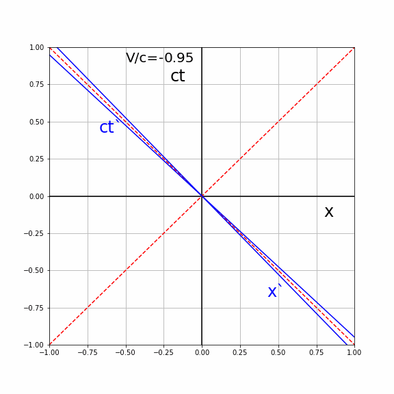
We plot the coordinate system of $S'$ (blue) in the coordinate system of S (black).

The time line of $S'$ in $S$ is given by the fact that $x'=0$ . From the LT we have $x'=\gamma (x-\frac{V}{c}ct)=0 \Rightarrow x=\frac{V}{c}ct$ . The angle $\alpha$ of the $ct'$ -line with the $ct$ axis is given by $\tan \alpha = \frac{V}{c}$ .
The space line of $S'$ in $S$ is given by the fact that $ct'=0$ . From the LT we have $ct'=\gamma (ct-\frac{V}{c}x)=0 \Rightarrow ct=\frac{V}{c}xt$ . The angle $\alpha$ of the $x'$ -line with the $x$ axis is given by $\tan \alpha = \frac{V}{c}$ .

Both lines of $S'$ make the same angle $\alpha$ with the coordinates axis of $S$ . They lie symmetric around the light line $x=ct$ (diagonal with $\alpha=45$ deg). The higher the speed $V$ the higher the angle and the closer the lines lie to the light line. See the animation below, where the $(ct',x')$ axis are plotted in the $(ct,x)$ diagram of $S$ for different values of $V/c$ .

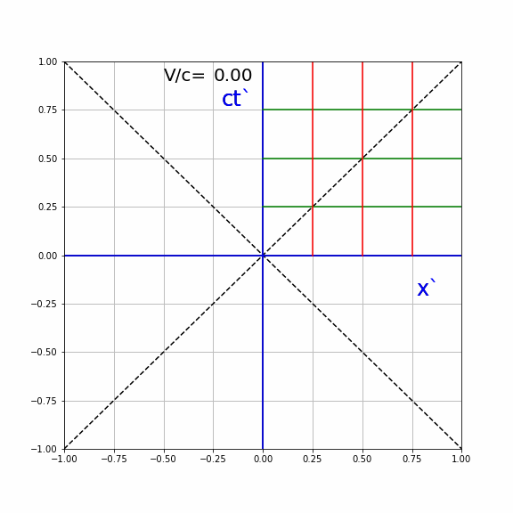
To further investigate how this plot can help us, let us consider lines of equal time in $S$ . These are just the lines perpendicular to the $ct$ -axis, and parallel to the $x$ -axis, as you expect. And of course, lines parallel to $ct$ , perpendicular to $x$ are lines of constant space coordinate.

For the frame of reference $S'$ that is only a bit different.

Lines of constant time in $S'$ are parallel to $x'$
Lines of constant space coordinate in $S'$ are parallel to $ct'$

With this information in hand, we can investigate how events are transferred from $S$ to $S'$ . We can graphically do a LT without the explicit computation.

In the animation below, we see the effect of different values of $V/c$ on the lines of constant $ct'$ and $x'$ as seen by $S$ . For clarity, these are only drawn for $V/c \geq 0$

4.4.1The ladder & barn revisited¶

We will now take a look back at the ladder and barn paradox. We had a barn of $10 \mathrm{m}$ wide and a ladder of $26 \mathrm{m}$ long (both measured in their rest frame). The ladder was moving towards the barn with high velocity. We start by drawing the barn $S$ (black) and ladder $S'$ (blue) coordinate systems in the Minkowski diagram. Now we add the barn world line into the diagram (light blue) with 2 lines of constant space coordinate (parallel to $ct$ ) in $S$ .

Now we can add the ladder to $S'$ . It has rest length of $26 \mathrm{m}$ and in the $(x',ct')$ plane it is a world line of constant space coordinate, therefore parallel to $ct'$ . The ladder itself is a line of constant time in $ct'$ and therefore parallel to $x'$ .

As the ladder moves (we move it parallel to $x'$ between the world lines) it will eventually enter the barn and hit the right door of the barn (dashed red line). This event is indicated by the space time point $A$ . For $S'$ the other end of the ladder is then still outside the barn at space time point $C$ . According to $S'$ the ladder does not fit into the barn.

When the ladder hits the right door for $S$ at space time point $A$ , he makes a measurement of the ladder. To this end we draw a line of constant time (dashed light blue, parallel to $x$ ) until it intersects the world line of the ladder at space time point $B$ . Observer $S$ measures that the ladder fits into the barn.

From this diagram it is obvious that the events $B$ and $C$ are not the same, therefore it is not strange that $S$ and $S'$ disagree about the outcome of the measurement. Both are right! But they would not be able to agree that both doors shut at the same time, to capture the ladder.

4.4.2The twin paradox¶

Let there be two twins, Alice and Bob. Bob leaves earth in a space ship with relativistic speed $\vec{v}$ , while Alice remains back home on earth. At some time Bob turns around, with $-\vec{v}$ and comes back to Alice. Based on time dilation Alice will argue that Bob is younger than she due to $\Delta T = \gamma \Delta T_0$ . For the $gamma$ -factor it does not matter if Bob is moving away or approaching as it is quadratic in the velocity. For each year she ages, her brother only ages $1/\gamma$ years. Bob can argue that due to the principle of relativity, he is at rest and his twin sister is moving away and then coming back, therefore she will be younger than he - and we have a paradox.

This paradox has two issues:

The principle of relativity is not applicable as Bob must turn around. This requires acceleration of his frame and breaks the symmetry of the problem.
Bob will be younger than Alice, due to the relativity of simultaneity changing around the turning point. We can see this by looking at the Minkowski-diagram below. Just before Bob is turning around, his line of simultaneity is $x'$ , but just after turning around his line of simultaneity is $x''$ . On the time line of Alice, Bob lines of simultaneity first is at point A, but then makes a jump around the turning point to B. Bob will be younger than Alice, by the length of this jump on her time line from A to B.

Extra: We symmetries the problem. Both Alice and Bob move in space ships away from each other at the same but opposite speed, then turn around and meet again. Who is older now?

Answer

They are the same age. You can now reason with symmetry even though both are accelerated. You can also draw the Minkowski-diagram similar to the above and see that both make the same “jump” in the time, and thus are the same age.

the rabbit and the turtle

We consider the relativistic race between the well-known rabbit ( $R$ ) with speed $v_R$ and his buddy turtle ( $T$ ) with speed $v_T<v_R$ . Both turtle and rabbit are point particles. To give turtle a chance, it does not need to run as far as rabbit $(L_T<L_R)$ . The distances are chosen such that an observer at rest (the audience) records that $R$ and $T$ finish at the same time.

Draw a Minkowski-diagram of the situation described above.
Indicate the following events in space time.
- $R$ finishes in his frame (A)
- $T$ finishes in his frame (B)
- In the frame of $R$ , when he finishes, the event where $T$ is then (C)
- In the frame of $T$ , when he finishes, the event where $R$ is then (D)
Who has won according to $R$ and who according to $T$ . Do they agree?

Solutions:

We start by drawing the audience frame with $(ct,x)$ and an equal time line for the finish of $R$ and $T$ . From that we draw the coordinate system of $R$ as $(ct_R,x_R)$ and of $T$ as $(ct_T,x_T)$ . As $v_T < v_R$ , the coordinate system $(ct_R,x_R)$ is closer to the light line. The length $L_R$ and $L_T$ follow as the intersections of $ct_R$ and $ct_T$ with the line of equal time for the audience.

These intersections are also directly the events A and B.

For the events C and D, we first draw from A a line of constant time for $R$ (parallel to $x_R$ ) and then look at the intersection with the world line of $T$ and mark it with C. The same for the event D. We draw a line parallel to $x_T$ of constant time for $T$ through B to see where $R$ is when $T$ finishes and mark it with D.

Both $R$ and $T$ agree that $R$ has won, but the audience does of course not agree.

moving particle

Consider a standard situations: $S'$ moving at $V/c=3/5$ with respect to $S$ . CLocks are synchronized at $ct'=ct=0$ when $x'=x=0$ .

According to $S$ , a particle is moving with $U/c=4/5$ over the x-axis. $S$ describes the trajectory of the particle as $x_p(ct) = \frac{U}{c}ct$ . In the animation below a Minkowski diagram is plotted as $S$ would do. The motion of $S'$ is made visible by the moving blue dot. Similarly, the pink dot shows the motion of the particle. The grey grid is giving coordinates according to $S$ . The black dashed lines show the $ct$ and $x$ coordinate of the particle as $S$ uses.

The green dashed lines is the grid of $S'$ translated to the world of $S$ . The pink dashed lines show the corresponding coordinates of the particle in the world of $S'$ : they intersect the $ct'$ and $x'$ axes at the position and time as $S'$ would use. Notice that the clock of $S'$ is indeed slow. Of course the $x'$ coordinate of the particle stays relatively small: $S'$ is ‘chasing’ the particle.

4.4.3Lines of invariant distance¶

We have seen that the length interval $ds^2$ is a Lorentz invariant. Therefore we can use it to also indicate corresponding time and space units in a Minkowski diagram for two moving observers. If we fix $ds^2$ then the equation $ds^2=c^2 dt^2-dx^2$ describes a hyperbola in $(ct,x)$ of the Minkowski diagram.

For $ds^2<0$ we find the corresponding space units (the interval is space-like), and for $ds^2>0$ the corresponding time units (the interval is time-like. All hyperbola have the light line $ds^2=0$ as asymptotes.

Circles are not circular??

We define a circle as the set of points (in a plane) that have the same distance to some given point $M$ . We can easily extend this to three dimensions: that the circle becomes the surface of a sphere. If we stick to Eucledian spaces, we can do this for any dimension: a spherical surface in n-dimensional space, is the collection of points with the same distance to a given point $M$ . Now the point has to be represented by $n$ coordinates. But our measure of distance follows the same inner-product as we use in 2 and three dimensions:

let $\{M_i\} \text{ with } i=1..n$ be a point in n-dimensional space. Then all points $\{X_i\} \text{ with } i=1..n$ that obey the rule

\sum_{i=1}^n ( X_i - M_i)( X_i - M_i) = R^2

(15)

form a spherical surface with distance $R$ to $M$ . The above rule is actually the inner product of $\vec{X} - \vec{M}$ : $(\vec{X}-\vec{M})\cdot (\vec{X} - \vec{M} ) = R^2$

Without loss of generality, we can chose the origin at $M$ . That simplifies notation: $\vec{X} \cdot \vec{X} = R^2$ is now the surface of a sphere of radius R with center $\mathcal{O}$ .

What if we leave our Eucledian space and go to the Minkowski space of special relativity? We still would define e circle as a set of point with the same distance to a given point. But now, our measure of distance is different. Let’s again take the origin as the central point. Then, we are looking for the set of point $\{ X^\mu \}_i$ such that $\vec{X} \cdot \vec{X} = R^2$ . This means:

X^0 X^0 - X^1 X^1 - X^2 X^2 - X^3 X^3 = R^2

(16)

Or, if we only consider $ct, x$ :

c^2t^2 - x^2 = R^2

(17)

These are the ‘circles’ in Minkowski $ct,x$ -space. Of course, we would have the tendency to call them hyperbola, as they have the mathematical expression of a hyperbola. But in fact, the interpretation in Minkowsi space would be that of circles, that is the collection of points with the same distance to the origin.

Note, that $R=0$ now does not reduce the set to a single point, but instead refers to the light lines. Second note: we do not have a problem here with negative distances. Thus if we take $R$ to be a pure imaginary number, we will still get hyperbola, but just rotated by 90°.

4.5LT as a rotation¶

This part is optional, but insightful.

You can think of the LT as a rotation of the 4 coordinates of Minkowski space time. Obviously it is not a “normal” rotation with a rotation matrix $R\in SO(n)$ as we encountered in change to polar coordinates.

The LT in matrix notation reads as follows with $\gamma = \frac{1}{\sqrt{1-\beta^2}}$ and $\beta=V/c$ .

\left ( \begin{array}{c} ct' \\ x' \\ y' \\z' \end{array} \right ) = \left ( \begin{array}{cccc} \gamma & -\gamma\beta & 0 & 0\\ -\gamma\beta & \gamma & 0 & 0\\ 0 & 0 & 1 & 0 \\ 0 & 0 & 0 & 1\\ \end{array} \right ) \left ( \begin{array}{c} ct \\ x \\ y \\z \end{array} \right )

(18)

The matrix transfers the space time coordinates between two observers moving with $V$ . From this it is clear that transferring between more than two observers $S\to S' \to S^{''} \to \dots$ can be done easily by multiplying the respective Lorentz transformation matrices into one overall LT. This must be possible, of course, as the LT is a linear transformation in space time $(ct,x)$ .

From the matrix notation it is also clear that for rotations around “different axis”, speeds in $x,y,z$ direction, the order of change of frame matters as matrix multiplication does not commute.

In 3D normal space, distance is persevered under rotation with $R\in SO(n)$ , in Minkowski space distance is preserved under Lorentz transformation which too is a rotation.

You can see the rotation clearer if we introduce the quantity rapidity $\alpha$ , which is defined as $\tanh \alpha \equiv \frac{V}{c}$ (a relativistic generalization of the modulus of the velocity. It goes from 0 for $v=0$ to $\infty$ for $v=c$ ). We will not use the rapidity except here, however, it is used for relativistic velocity decompositions. With $\tanh \alpha = \frac{V}{c}$ we can write the Lorentz transformation as (using $\gamma = \frac{1}{\sqrt{1-\tanh^2 \alpha}}=\cosh \alpha$ and $\gamma\beta=\frac{\tanh\alpha}{\sqrt{1-\tanh^2 \alpha}}=\sinh\alpha$ )

\left ( \begin{array}{c} ct' \\ x' \\ y' \\z' \end{array} \right ) = \left ( \begin{array}{cccc} \cosh\alpha & -\sinh\alpha & 0 & 0\\ -\sinh\alpha & \cosh\alpha & 0 & 0\\ 0 & 0 & 1 & 0 \\ 0 & 0 & 0 & 1\\ \end{array} \right ) \left ( \begin{array}{c} ct \\ x \\ y \\z \end{array} \right )

(19)

Notice the similarity to the rotation with sine and cosine.

With that LT is a rotation in hyperbolic space with “angle” $\alpha$ (where $\alpha$ is the rapidity), we identify the matrix as $L(\alpha)$ . That the hyperbolic functions appear should not be a surprise as they are equivalent to the sine and cosine for the circle, $(ct^2+x^2=1)$ , for the hyperbola $(ct^2-x^2=1)$ . Notice the relation to the inner products for standard and Minkowski space.

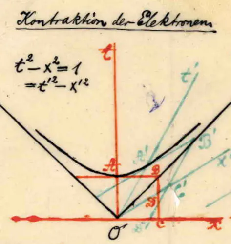
Minkowski made the sketch below to show that the Lorentz transformation is a rotation over a hyperbola not a circle as we were used to. The asymptotes of the hyperbola are given by the light lines.

The addition of velocities that we derived earlier is easy with this notation with rotations and rapidity $L(\alpha_1)L(\alpha_2)=L(\alpha_1+\alpha_2)$ . In terms of speeds this reads