Imagine we have two spaceships moving each with a speed of as shown below. What is the speed that either the red striped or yellow spaceships sees for the other spaceship speed?
We should, first of all realize, that the information regarding the velocity of the two spaceships is given by an observer who is neither in the red striped nor the yellow ship. We need to transform this information to an observer in the red striped or in the yellow ship.

Figure 1:Two spaceships approaching each other.
For the GT we have derived the velocity transformation to be
So, let’s translate our velocity information from the observer to someone in the red striped ship. The relative velocity between and the red ship is . Thus according to the observer in the red ship, , her velocity is , obviously.
However, she will denote the velocity of the yellow ship as . In the world of Galilei and Newton, this is no problem at all: velocities can be as big as you can imagine. However, in reality, this is not true. We have to use Special relativity if the velocities start to approach . It is not possible for any object to move faster than the speed of light, as we will see later.
In the above, we have only looked at the velocity component in the -direction. We have in addition found .
As our universe does not follow Galilei and Newton, we need to derive the transformation/addition formula for velocities with the LT. So let’s do it.
Velocity Transformation
Let us start from the definition of velocity (assuming we deal with constant velocities, so we don’t need to worry about differentiation and integration). We will denote velocities by to avoid confusion with , the relative velocity between the two observers.
Observer will write down:
We have left out the -component as that will be completely analogous to the -coordinate.
Observer will use similar definitions. How do these observers translate velocity information that they get from each other?
We need to use the LT to transform to :
and
From the last line it is clear that also the components of the velocity will be influenced by the transformation even though the relative motion between the two observers is only along the -direction. Substituting the expressions for the space and time difference into , we obtain
For the transverse components , we obtain due to the change of the time interval
In the limit of both formulas reduce to the Galilean Transformation as required. For and the combined velocity will stay smaller than . Check yourself that this is true!
The formula for the velocity transformation/addition are not so easy to remember. Later you will see how to derive them from the transformation properties of the 4-velocity, which is easy to remember.
For our example of the two approaching spaceships, we find for the speed of the yellow approaching the red ship
This is again smaller (in absolute sense) than . For the other ship we find of course the same, but with different sign.
Doppler effect
The Doppler effect is well-known from waves. You know it from daily life. If a car is passing you at high speed, the observed frequency (by you) is higher than the emitted frequency while the car is approaching, and smaller when it drives off.
Here we investigate the effect of a moving source that is emitting light with (electro-magnetic waves). This is one of the few cases where the relativistic case is easier than the classical effect. In the latter it matters if the source is moving or the medium. However, for EM-waves there is no medium (aether) as we have seen, which simplifies things.
Figure 2:Effect on sound waves due to motion.
For the case of an observer with speed and speed of sound in the medium and moving source (e.g. car) the classical formula of the frequency shift is
where for the stationary observer and medium, we have and for the moving observer and stationary source .
The origin of the observed frequency shift of a moving source is made visible in Figure 3. In the direction of motion, more wave maxima arrive per unit time, as the car is moving closer between two wave maxima. Consequently, the observer will count more maxima per unit time: the frequency is higher.
For the relativistic effect we consider a moving source with velocity moving with observer relative to . The frequency of the source is in the rest frame, with the period of the oscillation.

Figure 3:Observer S’ and source both moving with respect to S.
We now consider the situation for as shown in the figure below. The position of the source is indicated with the star .

We do know that according to , the proper frequency is and the proper period . Thus if a maximum is send at the next one will be at .
will denote the first maximum with time , but will have to take time dilation into account for the second one: . Note that these two time instants are the moments, according to when the two maxima are send, not when they are received by .
During this time interval the source moves from to . Thus, the distance that the second maximum has to travel is different from that of the first one, just like in the classical Doppler case.
We consider the two consecutive wave maxima that are emitted in and received in :
1 maximum in at , that is received in at . The additional time is needed for the light to travel from to the observer at the origin of .
2 maximum in at , is received in at .
To move further we split the velocity of the source into a radial component (in line to the observer in ) and a tangential part perpendicular . See Figure 5. If the distance then the distance .
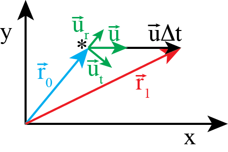
Note that we could drop the vector notation here from the exact relation above. Classically only the radial component is relevant as only the distance matters.
With this simplification on the distances we can compute
For the frequency in we now subtract the two arrival times
Rewriting this into a ratio of the emitted and received frequency, we obtain for the relativistic Doppler effect
Observe that the factor is of that means even for only tangential movement there is a Doppler shift.
Cosmic background radiation
The most well-known frequency shift is the red-shift from the expanding universe (probably disregarding speeding tickets resulting from radar measurements). Light coming from a star has a certain frequency as observed in the rest frame of the star. This frequency corresponds to a quantum mechanical drop in energy level. The photon emitted in this energy transition has a well known wave length and frequency. That is, of course, in the rest frame of the process. Anybody observing these photons while traveling with respect to the star will see a Doppler-shifted frequency. If the star is moving away from the observer, the wave length seems longer and thus the frequency lower: the light is shifted to the red end of the spectrum. If on the other hand the star is moving towards the observer, the waves seem compressed and the frequency detected is higher: the light is shifted to the blue end of the spectrum. Hence, astronomers talk about red sifted and blue shifted light.
The astronomer Edwin Hubble first found in the 1920s that the universe does not only consists out of our own galaxy, the milky way, but there must be (many) other galaxies, which were called nebula at that time. Second, he could show that all further away galaxies move away from us by measuring the Doppler shift of well-known emission lines of stars and their distance from periodic intensity variation of Cepheid Variable stars. It turned out that the distance of the galaxies was roughly linearly proportional to the red-shift which is again linearly related to the radial velocity as we derived. This is known now as Hubble’s law with the Hubble constant ( ). Further away galaxies move faster away, but why? And why is no galaxy approaching us?
At end of the 1920s Georges Lemaître applied Einstein general theory of relativity to cosmology and found that the universe must be expanding, while it started in a “primeval atom”, now known as the Big Bang. He could explain the red-shift relation from the expanding universe hypothesis.
The Big Bang theory was highly debated early on, in particular by Einstein, but is now fully accepted. The strongest experimental evidence was the discovery of the cosmic background radiation in 1965 (by accident).
The whole cosmos is nearly uniformly filled by a background radiation of about (wavelength in the m range) with small inhomogeneities as shown in the picture by the Planck satellite around 2013.
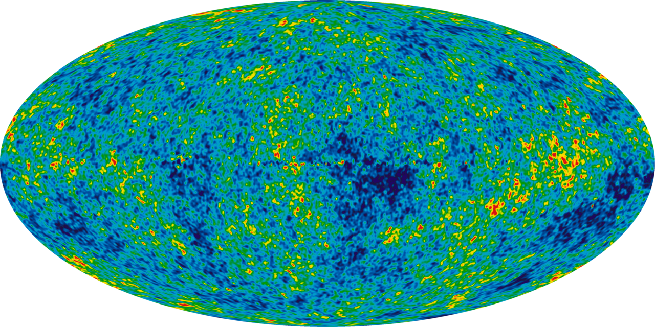
Figure 6:Background radiation in the universe as observed from earth.
By NASA / WMAP Science Team - http://
This radiation is the red shifted radiation from around 380,000 years after the Big Bang when the universe became transparent. At that time the temperature had dropped (due to the adiabatic expansion) to around 3000 K, at which protons and electrons can form stable hydrogen atoms . This event is called recombination. At higher temperatures photons are scattered from the free electrons (and protons) constantly, effectively the photons have a very short mean free path and the universe is opaque. At the recombination temperature all of a sudden the photon could travel without strong scattering, the universe was transparent. The cosmic background radiation that we measure today is the red-shifted version of this light. It gives us a glimpse of how the universe looked at that time. Apart from the background radiation there were no other light sources in the universe as stars had not formed yet, the Dark Ages of the universe began.
The red-shift here is actually caused by the expansion of the universe itself (the universe expands causing the photons’ wavelength to expand). NB: Time in cosmology is often given in units of red-shift (e.g. the red-shift for recombination is ).
Wavelength temperature relation
How can we relate the wavelength of electro-magnetic radiation to temperature?
Matter emits electro-magnetic radiation depending on its temperature. This relation is given by Planck’s law with which quantum mechanics started in 1900 as he considered black body radiation. The emitted spectral density per solid angle depends on the thermal energy and is given by
Here for the first time , Planck’s constant, was introduced to quantize energy packages of oscillation.
Phenomenologically, the relation between the peak of the spectrum and the temperature was found by Wien already earlier to be with Wien’s constant .
NB: If you buy a light bulb for a lamp, then a temperature is indicated on the packaging, e.g. for “warm white”, for “cool white” to describe the light color. Quantum physics at your local super market.
Source
import numpy as np
import matplotlib.pyplot as plt
import ipywidgets
from IPython.display import display

# Constants
h = 6.62607015e-34  # Planck constant, J*s
c = 3.0e8           # Speed of light, m/s
k = 1.380649e-23    # Boltzmann constant, J/K

# Wavelength range (from 1 nm to 3000 nm)
wavelengths = np.linspace(1e-9, 3000e-9, 1000)

# Planck's Law function with overflow protection
def planck(wavelength, T):
    exp_term = (h * c) / (wavelength * k * T)
    # Prevent overflow in the exponential function
    with np.errstate(over='ignore'):
        return (2.0 * h * c**2) / (wavelength**5) * np.where(exp_term < 700, 1/(np.exp(exp_term) - 1), 0)

# Visible spectrum range in meters
visible_start = 380e-9
visible_end = 750e-9

# Colors of the visible spectrum in the correct order from violet to red
colors = ['violet', 'indigo', 'blue', 'green', 'yellow', 'orange', 'red']
num_colors = len(colors)
wavelength_visible = wavelengths[(wavelengths >= visible_start) & (wavelengths <= visible_end)]
color_indices = np.linspace(0, len(wavelength_visible), num_colors + 1, dtype=int)

# Function to plot the Planck curve
def plot_planck_curve(T):
    spectral_radiance = planck(wavelengths, T)

    plt.figure(figsize=(10, 6))

    # Plot the Planck curve
    plt.plot(wavelengths * 1e9, spectral_radiance, label=f'T = {T} K')

    # Highlight the visible spectrum with rainbow bands
    for i in range(num_colors):
        plt.fill_between(wavelength_visible[color_indices[i]:color_indices[i+1]] * 1e9,
                         spectral_radiance[(wavelengths >= visible_start) & (wavelengths <= visible_end)][color_indices[i]:color_indices[i+1]],
                         color=colors[i])

    # Plot settings
    plt.xlim(0, 3000)
    plt.ylim(0, 4.5E14)
    plt.xlabel('Wavelength (nm)')
    plt.ylabel('Spectral Radiance')
    plt.title('Planck Curve')
    plt.legend()
    plt.grid(True)
    plt.show()

ipywidgets.interact(plot_planck_curve,T=(1,10000,100))