The concept of complex numbers has been introduced in the chapter on oscillations. It shows up in many places in physics, but isn’t often introduced simultaneously in math classes. Hence, we provide a brief introduction to complex numbers here.
The general idea
A complex number is a number that expresses both a quantity and a phase (angle) with a single number. Complex numbers are expressed in the form , where and are real numbers, and is the imaginary unit, which satisfies the equation (see below). The real part of the complex number is , and the imaginary part is . Complex numbers can be represented in the complex plane, where the horizontal axis represents the real part and the vertical axis represents the imaginary part. The magnitude of a complex number is given by , and the angle (or argument) is given by , see Figure 1.
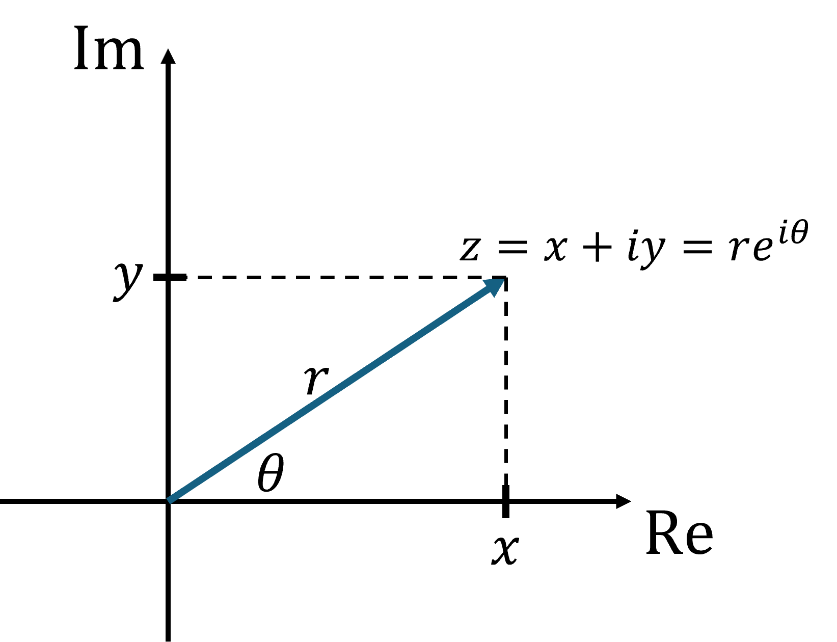
Figure 1:The complex plane, where the horizontal axis represents the real part and the vertical axis represents the imaginary part of a complex number.
Why using complex numbers is useful will be covered later, let’s first think a little more on representing complex numbers in the complex plane. Consider the following expression: multiplying by is the same as rotating by 90 degrees (in the complex plane). We can see this easily by taking the inner product. We take the complex number: :
If we think of this idea and imagine that we multiply twice by we get a 180 degree rotation, which is the same as multiplying by -1. This is consistent with the definition of as the square root of -1, or . Note that 180 degree is the same as the rotation of radians.
Python
We can use Python as a useful tool to help uncover characteristics of complex numbers. A complex number is given in python with the letter . By default real and imaginary numbers can be calculated - no additional python packages needed.
Source
import matplotlib.pyplot as plt
import numpy as np

data = np.array([2+2j, 4j, 4+1j, -4])
# extract the real and imaginary parts
x = data.real
y = data.imag

# plot the complex numbers
plt.scatter(x, y, color='k', marker='.')
plt.ylabel('Imaginary')
plt.xlabel('Real')
plt.show()
We can check that multiplying by is the same as rotating by 90 degrees (in the complex plane) is true in the python plot below.
Source
import matplotlib.pyplot as plt
import numpy as np

data = np.array([2+2j, 4j, 4+1j, -4])
data2 = data * 1j
# extract the real and imaginary parts
x, x2 = data.real, data2.real
y, y2 = data.imag, data2.imag

# plot the complex numbers
plt.scatter(x, y, color='k', marker='.')
plt.scatter(x2, y2, color='r', marker='.')
plt.ylabel('Imaginary')
plt.xlabel('Real')
plt.show()
Euler’s formula
From Figure 1 we see that the complex number can also be written as . Euler came up with a helpful way of rewriting this:
You could show that this is true in multiple ways, e.g. taking the series of the exponential function as well as of the cosine and sine function. However, we leave that to the math course.
Source
%pip install ipywidgets
import numpy as np
import matplotlib.pyplot as plt
from ipywidgets import interact, FloatSlider
from mpl_toolkits.mplot3d import Axes3D

def euler_plot(theta=0.0):
    t = np.linspace(0, 4*np.pi, 500)
    x = t
    y = np.cos(t)
    z = np.sin(t)

    fig = plt.figure(figsize=(8, 5))
    ax = fig.add_subplot(111, projection="3d")

    ax.plot(x, y, z, color="red", linewidth=2, label=r"$e^{i\theta}$")
    ax.plot(x, y, 0*t, color="green", linewidth=2, label=r"$\cos(\theta)$")
    ax.plot(x, 0*t, z, color="blue", linewidth=2, label=r"$i\sin(\theta)$")

    ax.scatter(theta, np.cos(theta), np.sin(theta), color="red", s=60)
    ax.scatter(theta, np.cos(theta), 0, color="green", s=60)
    ax.scatter(theta, 0, np.sin(theta), color="blue", s=60)

    ax.plot([theta, theta], [0, np.cos(theta)], [np.sin(theta), np.sin(theta)],
            color="gray", linestyle="--", linewidth=1)
    ax.plot([theta, theta], [np.cos(theta), np.cos(theta)], [0, np.sin(theta)],
            color="gray", linestyle="--", linewidth=1)

    ax.set_title(r"$e^{i\theta}=\cos(\theta)+i\sin(\theta)$", fontsize=16)
    ax.set_xlabel(r"$\theta$")
    ax.set_ylabel(r"$\mathrm{Re}[e^{i\theta}]$")
    ax.set_zlabel(r"$\mathrm{Im}[e^{i\theta}]$")

    ax.set_xlim(0, 4*np.pi)
    ax.set_ylim(-1.1, 1.1)
    ax.set_zlim(-1.1, 1.1)

    ax.view_init(elev=20, azim=-65)
    ax.legend()
    plt.show()

interact(
    euler_plot,
    theta=FloatSlider(
        value=np.pi,
        min=0,
        max=4*np.pi,
        step=0.05,
        description=r"$\theta$"
    )
)
cos(x) and sin(x)
Using Euler’s formula:
we can derive expressions for either the cosine or sine function. We replace replace with and consider that is an even function () and is an odd function ():
If we add (3) and (4), we get:
and if we subtract the two functions we get:
or, more frequently given as:
Integrating
Using complex numbers, we can make some integrals easier to solve (like sometimes switching to the frequency domain helps also in solving integrals). Below we provide two examples:
where we first have used (7). This becomes:
Rearranging and changing back to trigonometric functions we would obtain:
Let’s look at another difficult integral:
We can consider that the cosine is the real part of Euler’s formula and rewrite the integral:
The primitive of this function is much easier:
But we didn’t come here to make integrals easier, although it is a good idea to see how complex numbers may make your life as a physics student easier. The true reason why we introduced complex numbers was of their use in differential equations.
Solution to differential equations
The solution of a differential equation in which the second derivative is proportional to the negative of the function itself is harmonic oscillation:
We have seen before that the cosine and sine function may be written using Euler’s formula. Let us investigate how this would work with the equation above.
We propose the general solution
If we use (14) and our general solution we get:
Rearranging and reducing:
or , which is the same as (see oscillations) the angular frequency . Based on the initial conditions we can find the values of and .