Derivatives
There are multiple interpretations of what a derivative is:
Geometric: The derivative at a point gives the slope of the tangent line to the curve at that point.
Physical: The derivative represents the instantaneous rate of change, such as velocity being the derivative of position with respect to time.
Analytical: The derivative is defined as the limit of the average rate of change as the interval approaches zero.
Source
import numpy as np
import matplotlib.pyplot as plt

x = np.linspace(0,2*np.pi,500)
y = 2.3*np.sin(x)
dy_dx = np.gradient(y, x)


i = 70
x0 = x[i]
y0 = y[i]
slope = dy_dx[i]

tangent = y0 + slope * (x - x0)

plt.figure()
plt.plot(x,y)
plt.plot(x,dy_dx,'r--', label='derivative')
plt.plot(x,tangent,'b--',label='tangent')
plt.scatter(x0, y0, zorder=3,label='point of contact')
plt.ylim(-2.5,2.5)
plt.xlabel('x')
plt.ylabel('y')
plt.legend()
# plt.savefig('../derivative.png',dpi=450)
plt.show()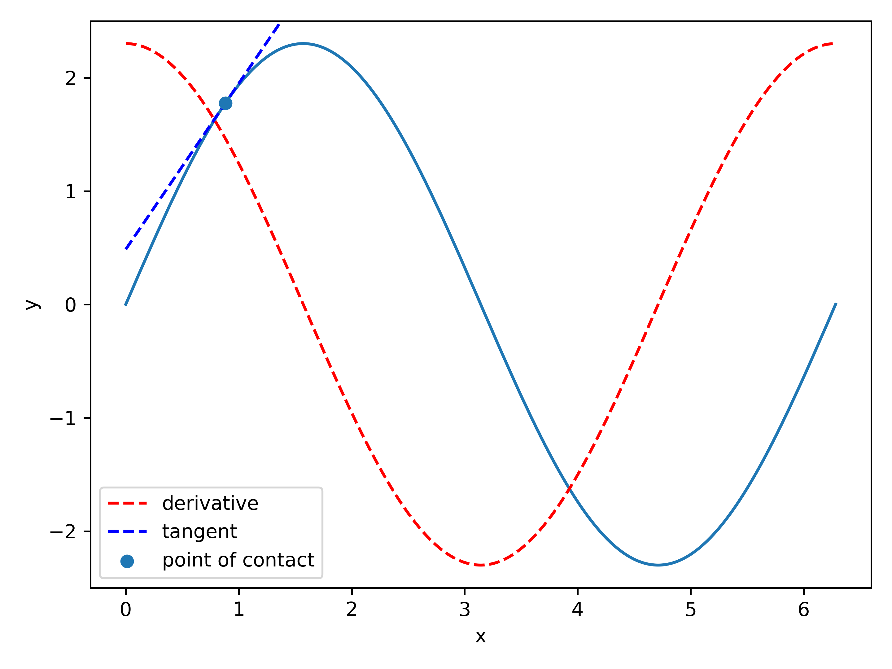
Figure 1:A sine function with both its derivative (a cosine function) and its tangent at a certain point.
In general the rate of change at a certain point can be taken using:
and the derivative the limit of
We now can calculate the rate of change of a given function, but we can calculate as well the exact value by taking the derivative. Below a list of some standard functions and their derivatives with respect to . The list is followed by mathematical rules that can be applied to calculate the derivative of more difficult functions.
List of standard derivatives
| function () | derivative () |
|---|---|
| 1 | |
| y | |
| () | |
Chain rule
A function with a function (like ) can be differentiated using the chain rule:
Product rule
A function that is the product of two functions and can be differentiated using the product rule:
A simple example would be differentiating where we know this could be written as and its derivative is . Using the product rule we get:
Quotient rule
The quotient rule is applied when differentiating a function that is the quotient of two functions and : . The derivative is then give by:
Summarized
| Function | Derivative |
|---|---|
Partial derivatives
Above we have only discussed derivatives of functions with one variable. However, many functions depend on multiple variables, e.g. . In such cases, we can compute the partial derivative with respect to one of the variables, treating the other variables as constants. Consider the function . The partial derivative of with respect to is computed as follows:
and with respect to :
Noted that in the first year physics course, you will encounter this as well as you often have to deal with uncertainties in multiple quantities. To find the total uncertainty, you will need to compute the partial derivatives of the function with respect to each variable.
Integration
The antiderivative (Dutch: primitieve) of a function is the function such that .
List of standard antiderivatives
Below is a list of some standard functions and their antiderivative with respect to .
| function () | antiderivative () |
|---|---|
| + C (for ) | |
| (for ) | |
| [1] |
Sum rule
In case where the antiderivative is (or can be) written in the form of two function, the sum rule can be applied:
Product rule
In case of two functions we can make use of the product rule, or integration by parts:
Substitution rule
When integrating the product of two functions, we may encounter the special case where one function is (up to a constant factor) the derivative of the other. In this situation, the substitution rule provides a straightforward way to evaluate the integral:
Line integrals
We encounter line integrals in the chapter on work. The amount of work done by a force field when moving an object along a path is given by the line integral:
We can visualize this by drawing the force field as arrows in space and the path as a curve. The line integral sums up the contributions of the force along the path, taking into account both the magnitude and direction of the force relative to the path. By looking whether the path goes with or against the force field, we can determine whether the work on the object or by the object.
In a conservative force field, such as gravity or electrostatic forces, the work done is path-independent and only depends on the initial and final positions.
Closed loop integrals
We encounter closed loop integrals in chapter ... There we see that a closed loop integral is the same as a line integral where the start and end point are the same. A closed loop integral is denoted as:
If we use again the idea of a conservative force field, we can see that in such a field the closed loop integral is always zero, as the work done going from point A to point B is exactly canceled out by the work done going back from point B to point A.
Curl, divergence and gradient
For two or three dimensional vector fields, the derivative can apply to all directions. For this, the nabla operator exists. In three dimensions, the nabla operator is a vector that takes the partial derivative along each coordinate:
The nabla operator can be applied to a scalar (gradient) or to a vector(field) using the dot or cross product (divergence and curl). We will discuss each of these below.
Note that some of the explanation below is better understood when looking at linear algebra first.
Gradient
We have seen the use of gradient in chapter 3. The gradient of function is . It creates a vector that indicates the directions in which increases or decreases:
Curl
The curl is used in the chapter on work and energy, specifically in the context of assessing whether a force field is conservative (if so, the path from A to B does not matter on the amount of work that is done). The curl of a vector field is denoted as . In mathematical terms, it provides a measure of the rotation (or swirling strength) of the field at a given point. A zero curl indicates that the field is irrotational, which is a characteristic of conservative fields. To get a better conceptual understanding, we can inspect the two fields below. The left is clearly rotating around the center, while the right one is not as all vectors point to the same direction (0,0). Hence, we expect that if we take the curl of the left field, it will be non-zero, while for the right field it will be zero.
Source
import numpy as np
import matplotlib.pyplot as plt


def F1(x, y):
    return y, -x

def F2(x, y):
    r = np.sqrt(x**2 + y**2)
    r = np.where(r == 0, 1e-10, r)  # Avoid division by zero
    return -x / r**3, -y / r**3

N = 7
xlim=(-2, 2)
ylim=(-2, 2)
x = np.linspace(xlim[0], xlim[1], N)
y = np.linspace(ylim[0], ylim[1], N)
X, Y = np.meshgrid(x, y)

Fx1, Fy1 = F1(X, Y)
Fx2, Fy2 = F2(X, Y)

fig, (ax1, ax2) = plt.subplots(2, 1, figsize=(5, 10))
ax1.quiver(X, Y, Fx1, Fy1)
ax2.quiver(X, Y, Fx2, Fy2)

ax1.set_xlabel("x")
ax1.set_ylabel("y")
ax1.set_xlim(xlim)
ax1.set_ylim(ylim)
ax2.set_xlabel("x")
ax2.set_ylabel("y")
ax2.set_xlim(xlim)
ax2.set_ylim(ylim)
plt.show()
Mathematically, the curl in three dimensions is defined as:
where , , and are the unit vectors in the x, y, and z directions, respectively, and , , and are the components of the vector field . Note that the outcome of taking the curl at a point returns a vector (or taking the curl of the vector field results in another vector field).
Divergence
The divergence of a vector field is denoted by . It quantifies the magnitude of a source or sink at a given point in the field (e.g. how strong a point is attracting or repelling). A positive divergence indicates a source (where field lines are diverging, such as the electric field -field around a proton), while a negative divergence indicates a sink (where field lines are converging, such as the electric field -field around an electron). Mathematically, the divergence in three dimensions is defined as:
where , , and are the components of the vector field . Note that taking the divergence at a point returns a scalar value, not a vector.