Worked examples
The earth’s gravitational force acting on the moon
Given the following:
what is the gravitational acceleration due to the earth’s gravitational force acting on the moon?
When you stand at the earth, your body is attracted to the center of the earth. This is the same for the moon: it is pulled towards the earth’s center. We know that the gravitational force is inversely proportional to the square of the distance between the two objects.
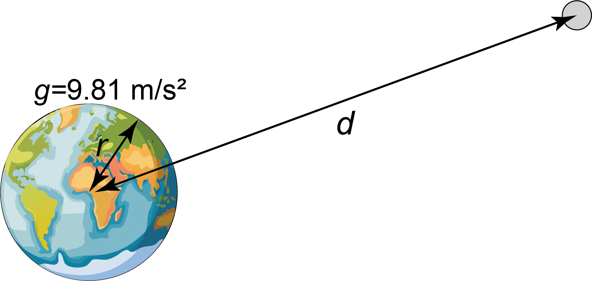
Figure 1:A schematic of the situation.
The distance from the center of the earth to the moon is times as large as the distance from us to the center of the earth. Hence, we expect the gravitational force to be 60.32 as small.
The gravitational acceleration due to the earth’s gravitational force acting on the moon is approximately .
What we might recall from high school is . For a circular orbit, with , we can rewrite this as and thus . Slotting in our numbers we get seconds, which is approximately , which is the correct orbital period of the moon around the earth.
What we learn from this is that we sometimes don’t need to know the exact formula and all the constants to solve a problem, sometimes ratios are sufficient.
Exercises
### Your code### Your codeSolutions
Solution to Exercise 1
Using the same data as in the previous example, plus
.
nearest point to the moon: .
farthest point from the moon: .
This thus means that the nearest point of the earth to the moon is pulled more strongly towards the moon than the center of the earth: explaining the first tide. The farthest point of the earth from the moon is pulled less strongly towards the moon than the center of the earth allowing the water to rise there more than at the center of the earth: explaining the second tide.
Note as well that the gravitational acceleration due to the moon’s gravitational force acting on the earth is much less than the gravitational acceleration due to the earth’s gravitational force acting on the moon. Still, as we will see in the next chapter, the gravitational force is the same!
Solution to Exercise 2
Solution to Exercise 3
The physical constants , and have the following numerical values and SI-units:
Note: the value of is precise, i.e. by definition given this value. The second is defined via the frequency of radiation corresponding to the transition between the two hyperfine levels of the ground state of the caesium-133 atom.
If we want to combine these three units into a length scale, , we try the following:
What we mean here, is that the units of the quantities (denoted by [.]) left and right should be the same. Thus, we get:
We try to find such that the above equation is valid. We can write this equation as:
If we split this into requirements for m, kg, s we get:
From the second equation we get . Substitute this into the first and third and we find:
Add these two equations: and thus and .
So if we plug these values into our starting equation we see:
We can repeat this for energy, :
Note: the unit of energy, [J] needs to be written in terms of the basic units: .
The outcome is: , , and thus our energy is:
Solution to Exercise 4
The size of a duck is on the order of . It flies at a speed of about , that is . Thus we compute for the Reynolds number of a flying duck:
Clearly, the inertial force is dominant.
What about a swimming duck? Now the velocity is much smaller: . The viscosity of water is and the water density is . We, again, calculate the Reynolds number:
Hence, also in this case inertial forces are dominant. This perhaps comes as a surprise, after all the velocity is much smaller and the viscosity much larger. However, the water density is also much larger!
For a swimming bacterium the numbers change. The size is now about and the velocity (numbers taken from internet). That gives:
and we see that here viscous forces are dominating.
For an oil tanker the Reynolds number is easily on the order of 108. Obviously, viscous forces don’t do much. An oil tanker that wants to slow down cannot do so by just stopping the motors and let the drag force decelerate them: the Reynolds number shows that the viscous drag is negligible compared to the inertial forces. Thus, the tanker has to use ots engines to slow down. Again the inertia of the system is so large, that it will take a long time to slow down. And a long time, means a long trajectory.
For the flow of water through a (circular) pipe the Reynolds number uses as length scale the pipe diameter. We can relate the velocity of the water in the pipe tot the total volume that is flowing per second through a cress section of the pipe:
Thus we can also write as:
If for the pipe flow, we have:
with and we find: and .
Solution to Exercise 5
Solution to Exercise 6
# Moving a box

## Importing libraries
import numpy as np
import matplotlib.pyplot as plt


part_4 = 1 # Turn to 0 for first part

## Constants
m = 2 #kg
F = 30 #N
g = 9.81 #m/s^2
theta = np.deg2rad(10) #degrees

mu = 0.02
F_N = m*g*np.cos(theta) #N

## Time step
dt = 0.01 #s
t = np.arange(0, 10, dt) #s
t_F_stop = 0.5

## Initial conditions
x = np.zeros(len(t)) #m
v = np.zeros(len(t)) #m/s


## Loop to calculate position and velocity
for i in range(0, len(t)-1):
    if t[i] < t_F_stop:
        a = F/m - g*np.sin(theta) - F_N*mu*np.where(v[i] != 0, np.sign(v[i]), 0)*part_4
    else:
        a = -g*np.sin(theta) - F_N*mu*np.where(v[i] != 0, np.sign(v[i]), 0)*part_4
    v[i+1] = v[i] + a*dt
    x[i+1] = x[i] + v[i]*dt

## Plotting results
figs, axs = plt.subplots(1, 2, figsize=(10, 5))

axs[0].set_xlabel('Time (s)')
axs[0].set_ylabel('Velocity (m/s)')
axs[0].plot(t, v, 'k.', markersize=1)


axs[1].set_xlabel('Time (s)')
axs[1].set_ylabel('Position (m)')
axs[1].plot(t, x, 'k.', markersize=1)


plt.show()
Solution to Exercise 7
# Simulation of a base jumper

## Importing libraries
import numpy as np
import matplotlib.pyplot as plt

## Constants
A = 0.7 #m^2
m = 75 #kg
k = 0.37 #kg/m
g = 9.81 #m/s^2

## Time step
dt = 0.01 #s
t = np.arange(0, 12, dt) #s

## Initial conditions
z = np.zeros(len(t)) #m
v = np.zeros(len(t)) #m/s
z[0] = 300 #m

## Deploy parachute
A_max = 42.6 #m^2
t_deploy_start = 2 #s
dt_deploy = 3.8 #s

## Loop to calculate position and velocity
for i in range(0, len(t)-1):
    F = - m*g - k*A*abs(v[i])*v[i]  #N
    v[i+1] = v[i] + F/m*dt #m/s
    z[i+1] = z[i] + v[i]*dt #m
    # Check if the jumper is on the ground
    if z[i+1] < 0:
        break
    # Deploy parachute
    if t[i] > t_deploy_start and t[i] < t_deploy_start + dt_deploy:
        A += (A_max - A)/dt_deploy*dt

## Plotting results
figs, axs = plt.subplots(1, 2, figsize=(10, 5))

axs[0].set_xlabel('Time (s)')
axs[0].set_ylabel('Velocity (m/s)')

axs[0].plot(t, v, 'k.', markersize=1, label='numerical solution')
axs[0].vlines(t_deploy_start, v[t==t_deploy_start],0, color='gray', linestyle='--', label='parachute deploy')

axs[0].legend()

axs[1].set_xlabel('Time (s)')
axs[1].set_ylabel('Position (m)')

axs[1].plot(t, z, 'k.', markersize=1)
axs[1].vlines(t_deploy_start, 150,300, color='gray', linestyle='--', label='parachute deploy')


plt.show()
Solution to Exercise 8
import numpy as np
import matplotlib.pyplot as plt

F = 49/3
m1 = 1
dt = 0.001
t = np.arange(0, 100, dt) # s

x1 = np.zeros(len(t)) # m
x1[0] = 3
y1 = np.zeros(len(t)) # m
vx = 0
vy = 7


for i in range(0, len(t)-1):
    ax = -F*(x1[i]-0)/np.sqrt(x1[i]**2 + y1[i]**2)/m1
    ay = -F*(y1[i]-0)/np.sqrt(x1[i]**2 + y1[i]**2)/m1
    vx = vx + ax*dt
    vy = vy + ay*dt
    x1[i+1] = x1[i] + vx*dt
    y1[i+1] = y1[i] + vy*dt


plt.figure(figsize=(4,4))
plt.plot(x1, y1, 'k.', markersize=1)
plt.xlabel('x (m)')
plt.ylabel('y (m)')
plt.show()
Experiments
Exercise from Idema, T. (2023). Introduction to particle and continuum mechanics. Idema (2023)
- Idema, T. (2023). Introduction to particle and continuum mechanics. TU Delft OPEN Publishing. 10.59490/tb.81