Newton must have realized that his analysis of the Kepler laws was not 100% correct. After all, the sun is not fixed in space and even though its mass is much larger than any of the planets revolving it, it will have to move under the influence of the gravitational force by the planets. Take for example, the sun and earth as our system. By the account of Newton’s third law, the Earth exerts also a force on the Sun. Therefore, the Sun has to move as well; thus, we must revisit the Earth-Sun analysis and incorporate that the Sun isn’t fixed in space.
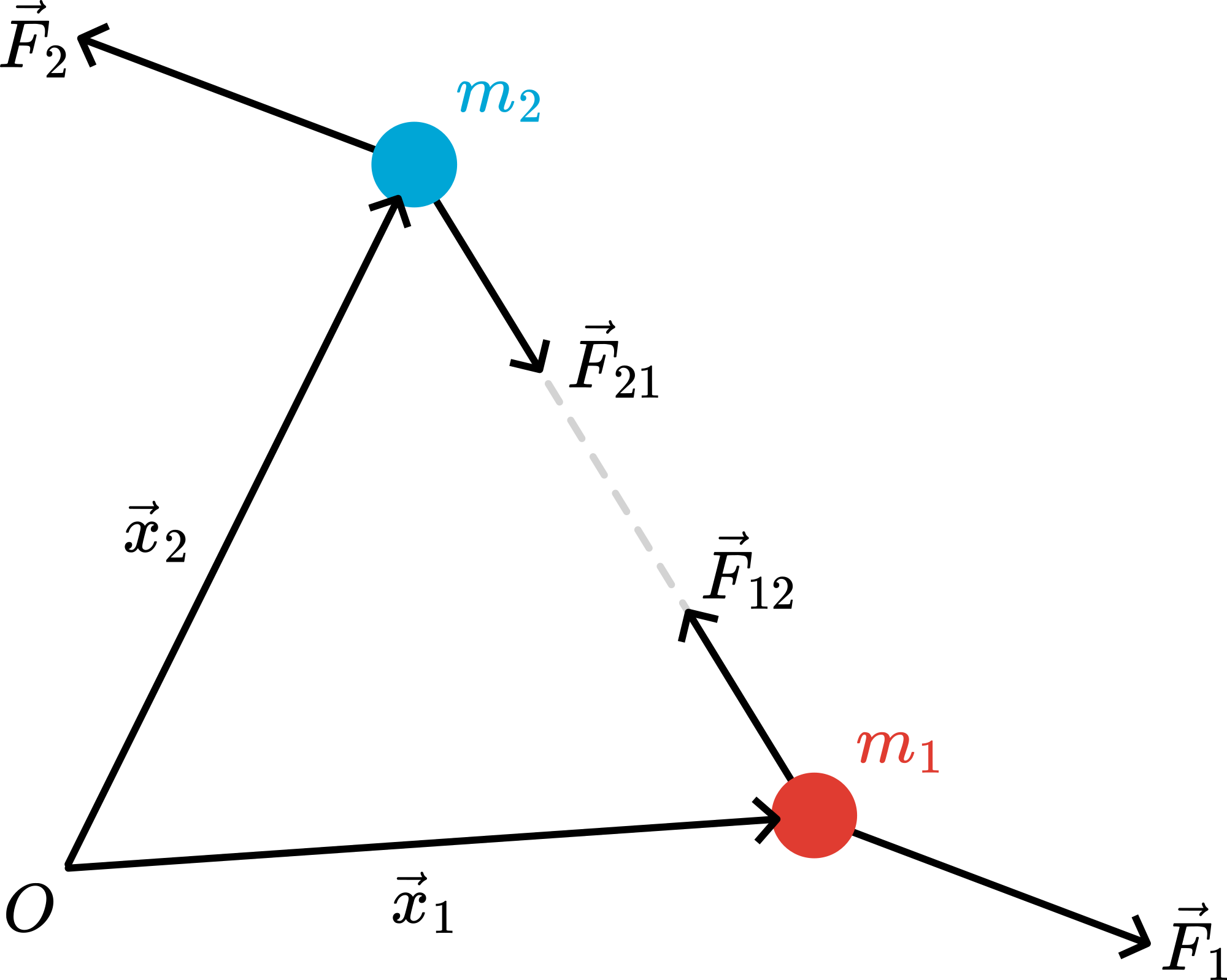
Figure 1:Two-particle system, with an action/reaction pair of forces.
The two-body problem is stated hereby as:
Particle feels an external force and an interaction force from particle two, . Similarly for particle : it feels an external force and an interaction force from particle one, .
Consider the situation in the figure:
Add the two equations and use N3: :
with . In words, it is as if a particle with (total) momentum responds to the external forces but does not react to internal forces (the mutual interaction).
8.1Center of Mass
It is now logical to assign the total mass to this fictitious particle. It has momentum which we can also couple to its mass and assign a velocity to it such that . Furthermore, if this fictitious mass has velocity , we can also assign a position to it. After all, , which gives us the recipe for the position .
Its velocity and position then follow as:
In the last equation, we have an integration constant in the form of a vector, . We are free to choose it as we want: its precise value does not affect the velocity nor the momentum of our fictitious particle.
It makes sense, to choose: and thus define as position of the particle:
Why?
We have a few arguments:
- if the particles are actually each half of a real particle, we obviously require that is the position of the real particle.
- If the particles are separate by a small distance, we would like to have the fictitious particle somewhere in between the two. Moreover, if the two particles are identical, it makes sense to have the fictitious particle right in between them: the system is symmetric.
Where, in general is the position ? That can be easily seen from the figure below.
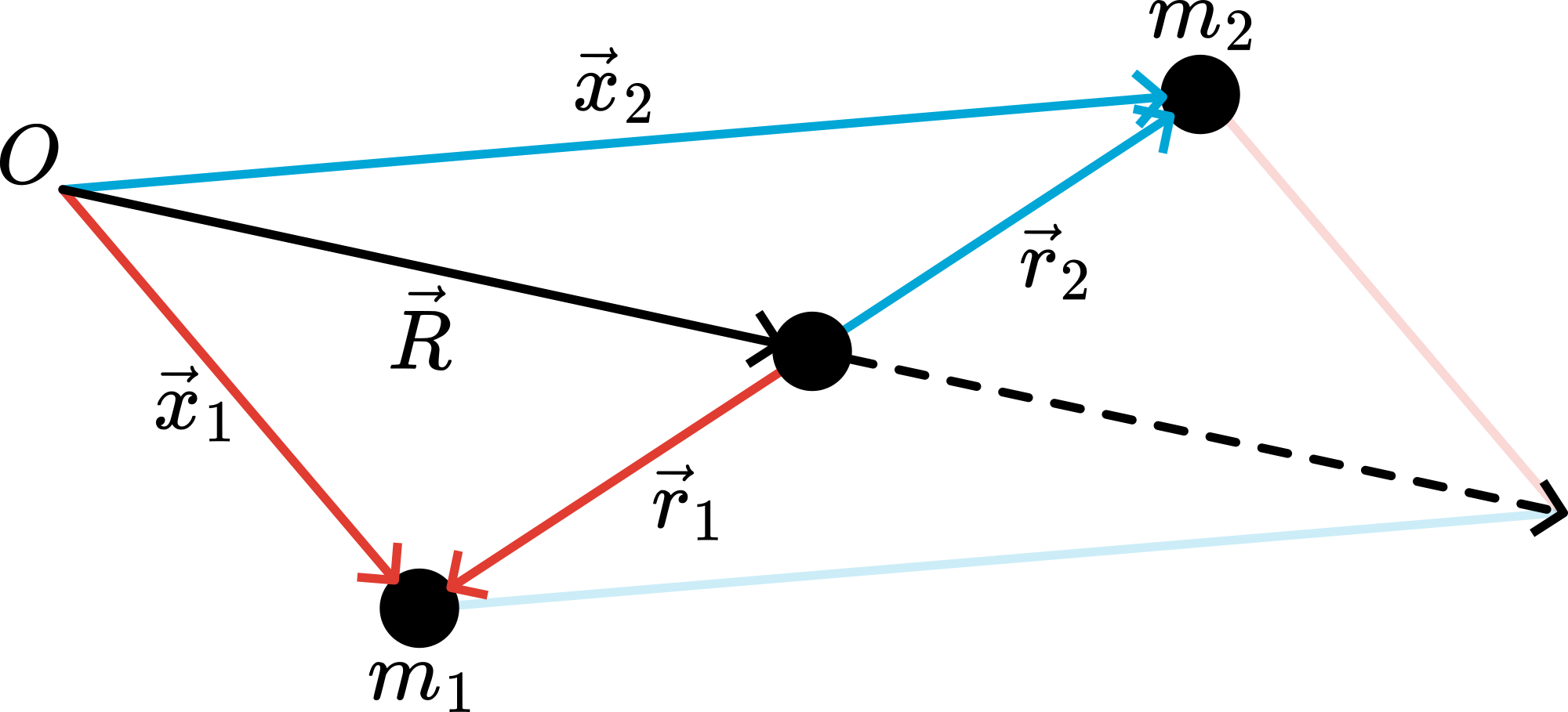
Figure 2:Center of Mass and relative coordinates.
We rewrite the definition of :
Thus, the last part of the above equation tells us: first go to and then, ‘walk’ a fraction of the line connecting and . If you have done that, you are at position .
Note: if this recipe indeed brings us right between the two particles.
Further note: the position of is always on the line from to . If is much larger than , it will be located close to and vice versa.
We call this position the center of mass, or CM for short. Reason: if we look at the response of our two particle system to the forces, it is as if there is a particle at position that has all the momentum of the system.
It turns out to be convenient to define relative coordinates with respect to the center of mass position (see also the figure above):
Via the external forces, we can ‘follow’ the motion of the center of mass position, i.e. . From the CM as new origin, we can find the position of the two particles.
A helpful rule is found from:
This has an important consequence: if we know , we know , and vice versa. Note: the directions of and are always opposed and the center of mass is located somewhere on the connecting line between and .
Note 2: in the case of no external forces and only internal forces the CM moves according to N1 with constant velocity .
8.2Energy
In terms of relative coordinates, we can write the kinetic energy as a part associated with the CM and a part that describes the kinetic energy with respect to the CM, i.e., ‘an internal kinetic energy.’
For the potential energy, we may write:
With the potential related to the external force on particle and the potential related to the mutual interaction force from particle exerted on particle (assuming that all forces are conservative).
8.3Angular Momentum
The total angular momentum is, like the total momentum, defined as the sum of the angular momentum of the two particles:
We can write this in the new coordinates:
We find: that the total angular momentum can be seen as the contribution of the CM and the sum of the angular momentum of the individual particles as seen from the CM.
8.4Reduced Mass
Suppose that there are no external forces. Then the equation of motion for both particles reads as:
If we divide each equation by the corresponding mass and subtract one from the other we get:
Note that the interaction force is a function of the relative position of the particles, i.e., .
Introduce , then we obtain:
As a final step, we introduce the reduced mass :
And we can reduced the two-body problem to a single-body problem, by writing down the equation of motion for an imaginary particle with reduced mass.
If we have . This is not surprising: when is much larger than , it will look like is not changing its velocity at all. Or seen from the CM: is appears to be not moving. In this case, we can ignore particle 1 and replace it by a force coming out of a fixed position.
8.4.1Back to the Two-Body Problem
Once we solved the problem for the reduced mass, it is straightforward to go back to the two particles. It holds that:
Thus, if we have solved the motion of the reduced particle, then we can quickly find the motion of the two individual particles (seen from the CM frame).
8.5Kepler Revisited
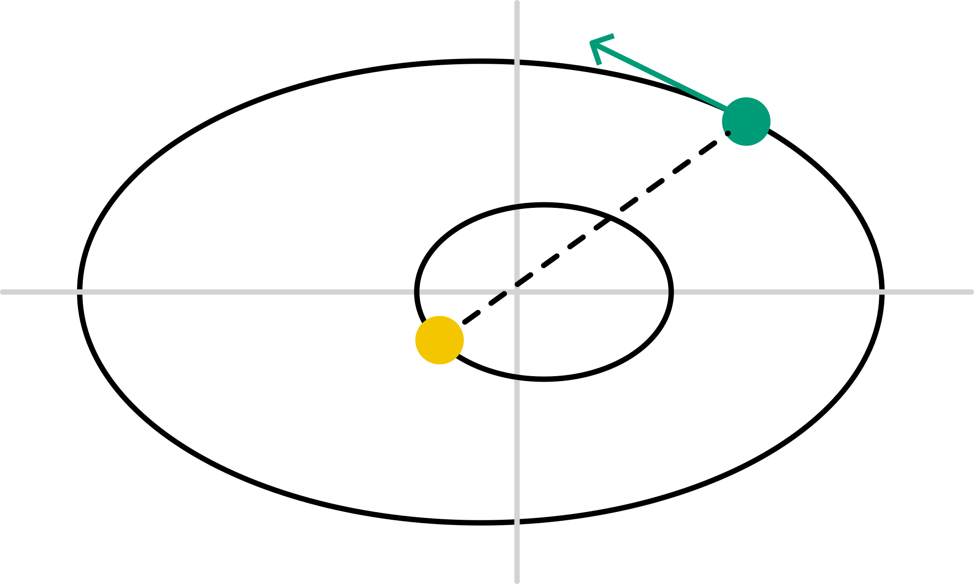
Figure 3:Kepler revisited.
Now that we have seen how to deal with the two-body problem, we can return to the motion of the Earth around the Sun. This is obviously not a two-body problem, but a many-body problem with many planets.
However, we can approximate it to a two-body problem: we ignore all other planets and leave only the Sun and Earth. Hence, there are no external forces. Consequently, the CM of the Earth-Sun system moves at a constant velocity. And we can take the CM as our origin.
We have to solve the reduced mass problem to find the motion of both the Earth and the Sun:
Note: this equation is almost identical to the original Kepler problem. All that happened is that on the left hand side got replaced by .
Everything else remains the same: the force is still central and conservative, etc.
8.5.1Where is the CM located?
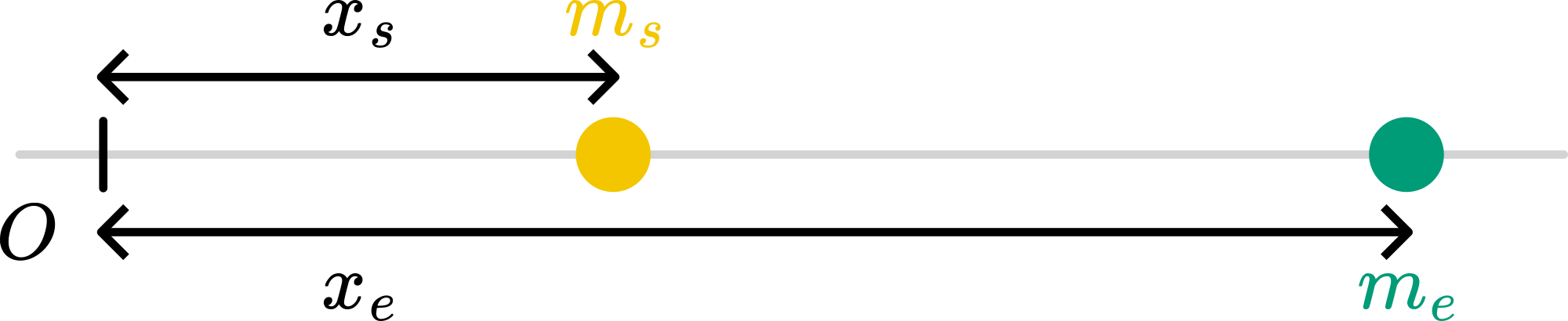
Figure 4:Position of CM in the sun-earth system.
We can easily find the center of mass of the Earth-Sun system. Chose the origin on the line through the Sun and the Earth (see fig.)
In other words: the Sun and Earth rotate in an ellipsoidal trajectory around the center of mass that is 450 km out of the center of the Sun. Compare that to the radius of the Sun itself: km. No wonder Kepler didn’t notice. The common CM and rotation point is called Barycenter in astronomy.
8.5.2Exoplanets
However, in modern times, this slight motion of stars is a way of trying to find orbiting planets around distant stars. Due to this small ellipsoidal trajectory, sometimes a star moves away from us, and sometimes it comes towards us. This moving away and towards us changes the apparent color of the light emission of molecules or atoms by the Doppler effect. This is a periodic motion, which lasts a ‘year’ of that solar system. Astronomers started looking out for periodic changes in the apparent color of the light of stars. One can also look for periodic changes in the brightness of a star (which is much, much harder than looking at spectral shifts of the light). If a planet is directly between the star and us, the intensity of the starlight decreases a bit. And they found one, and another one, and more and hundreds... Currently, more than 5,000 exoplanets have been found.
Figure 5:Changing color of star light due to a period motion induced by a planet orbiting the star (animation from NASA ).
Figure 6:Changing intensity of star light due to a period passage of a planet orbiting the star (animation from NASA).
8.6Many-Body System
We have seen that we could reduce the two-body problem of sun-earth to a single body question via the concept of reduced mass. But that this strategy does not work for 3, 4, 5, ... bodies.
8.6.1Linear Momentum
We can, however, find some basic features of -body problems. In the figure, a collection of interacting particles is drawn.
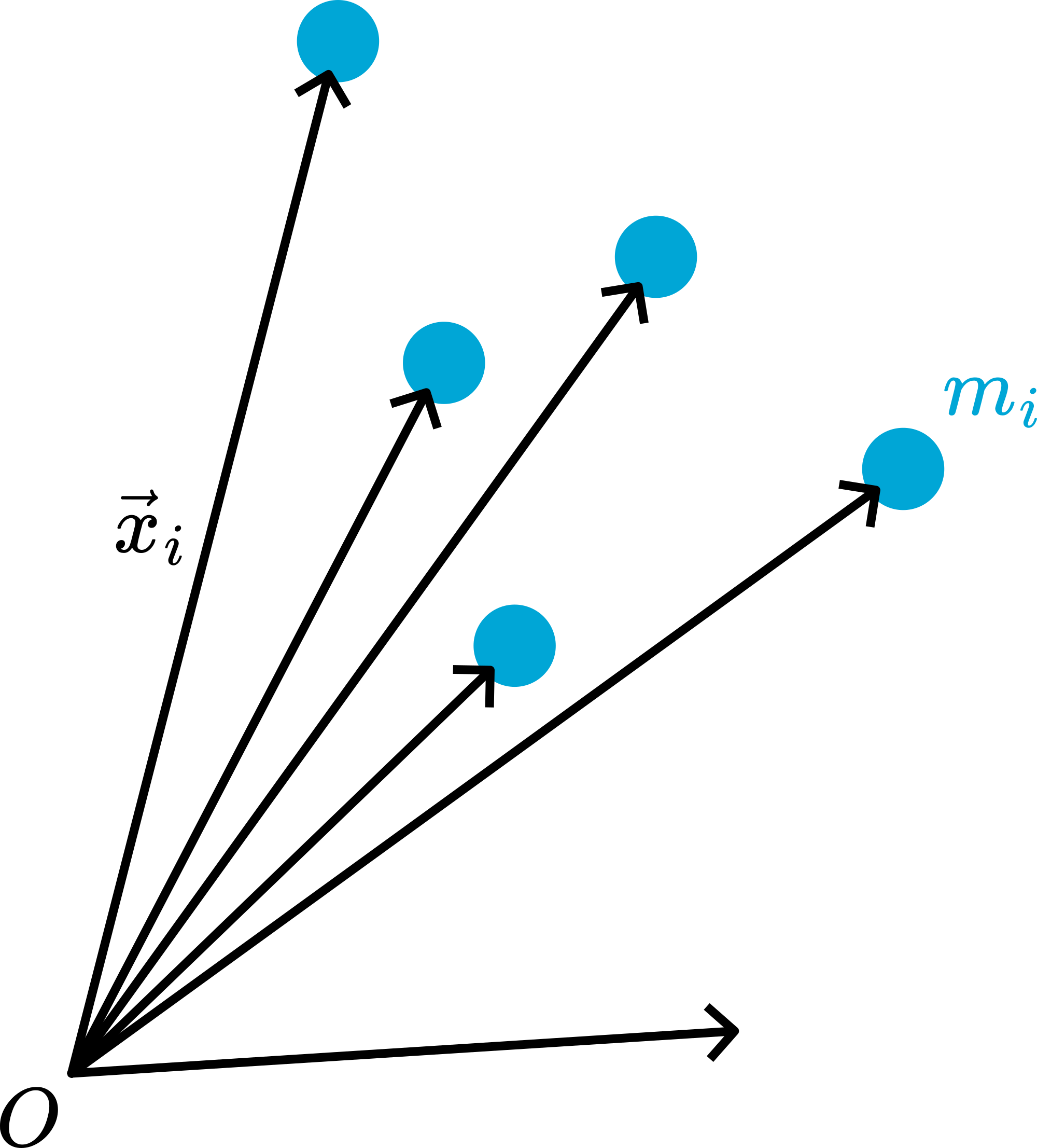
Figure 7:Many particle system.
Each particle has mass and is at position . For each particle, we can set up N2:
Summing over all particles and using that all mutual interaction forces form “action = -reaction pairs”, we get:
The second part can be written as:
In other words: the total momentum changes due to external forces. If there are no external forces, then the total momentum is conserved. This happens quite a lot actually, if you consider e.g. collisions or scattering.
8.6.2Center of Mass
Analogous to the two-particle case, we see from the total momentum that we can pretend that there is a particle of total mass that has momentum , i.e., it moves at velocity and is located at position:
Continuing with the analogy, we define relative coordinates:
and have a similar rule constraining the relative positions:
8.6.3Energy
In terms of relative coordinates, we can write the kinetic energy as a part associated with the center of mass and a part that describes the kinetic energy with respect to the center of mass, i.e., ‘an internal kinetic energy’.
For the potential energy, we may write:
with the potential related to the external force on particle and the potential related to the mutual interaction force from particle exerted on particle (assuming that all forces are conservative).
8.6.4Angular Momentum
The total angular momentum is, like the total momentum, defined as the sum of the angular momentum of all particles:
We can write this in the new coordinates:
Again, we find that the total angular momentum can be seen as the contribution of the center of mass and the sum of the angular momentum of all individual particles as seen from the center of mass.
The N-body problem is, of course, even more complex than the three-body problem. If we can solve it, it will be under very specific conditions only. However, a numerical approach can be done with great success. Moreover, current computers are so powerful that the system can contain hundred, thousands of particles up to billions depending on the type or particle-particle interaction.
All kind of computational techniques have been developed and various averaging techniques are employed in statistical techniques are introduced from the start. the reason is often, that a particular ‘realisation’ of all positions and velocities of all particles is needed nor sought for. A system is at its macro level described by averaged properties, the exact location of the individual atoms is not needed. You will find applications in cosmology all the way to molecular dynamics, trying to simulate the behavior of proteins or pharmaceuticals.