
Periodic Motion
There are many, many examples of periodic systems. We see them in physics, like the orbit of planets around their star. We find them in biology (like the predator-prey systems), in chemistry (oscillating reactions like the Belousov-Zhabotinsky reaction), and in economics (like demand-supply fluctuations). They show up in daily life: the day-night rhythm, the tides, children on a swing, your heart-beat. Periodic motions are by definition motions that repeat themselves after a fixed period of time, usually called ‘the period’.
A specific class of periodic motion is known as oscillatory motion, or simply oscillations. All oscillations are periodic, but not all periodic motions are oscillations. An oscillation involves movement back and forth around an equilibrium position. It is typically caused by a restoring force: a force that acts to return the system to equilibrium (in case of the mass spring system: ). However, due to inertia, the system overshoots this position. The restoring force then reverses direction, pushing the system back again, leading to continued oscillation.
A few simple examples will illustrate the above.
The merry-go-round
The merry-go-round (Figure 2) is a periodic motion, but not an oscillation. The seats go round in a circular, periodic motion but there is no back & forth. This is in contrast to a swing. That is also a periodic motion, but it has the back and forth as well as a restoring force, which in this case is gravity.
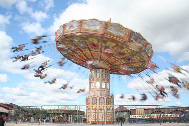
Figure 2:Spinning carousel. By Oxana Mayer, from Wikimedia Commons, licensed under CC BY-SA 2.0.
Rabbits and Foxes
As an example of a dynamic system that is periodic, we will take a look at the so-called predator-prey systems. These are well-known in biology and provide an interesting case. The idea is simple: the populations of rabbits growth as they multiply quickly. The idea in the prey-predator model is that growth rate is proportional to the population itself. For the rabbits that means that the derivative of the population of rabbits (with respect to time) is positive. If there are no foxes, the rabbit population will grow exponentially. Of course, in the real world that doesn’t happen as sooner or later, the rabbits will ran out of food, resulting in starvation. However, we will assume here, that food is not limiting: but the number of foxes is. They stop the rabbit population from unbounded increasing. The more rabbits there are, the easier the foxes find food and the more foxes will survive childhood. A simple model reads as follows:
here and represent the rabbit and fox population, resp. is the growth rate of the rabbits: the more rabbits, the larger the offspring. The higher the more babies per rabbit. , on the other hand, represents the effectiveness of the hunting foxes: the larger this value the more rabbits they kill. Of course: more rabbits, but also more foxes also means more kills. Similar arguments apply to and . Note that the term with carries a negative sign: the net increase of the fox population is negative if there is insufficient food, that is, by itself more foxes die then that are born if there is no food.
This is clearly a coupled and dynamic system. It is non-linear due to the product , making it much more difficult to solve analytically then linear versions. In literature, this kind of system is known as Lotka-Volterra or prey-predator models. Below is a plot of the numerical solution of the rabbit and fox population (for and initial conditions (, ) = (80, 2)).
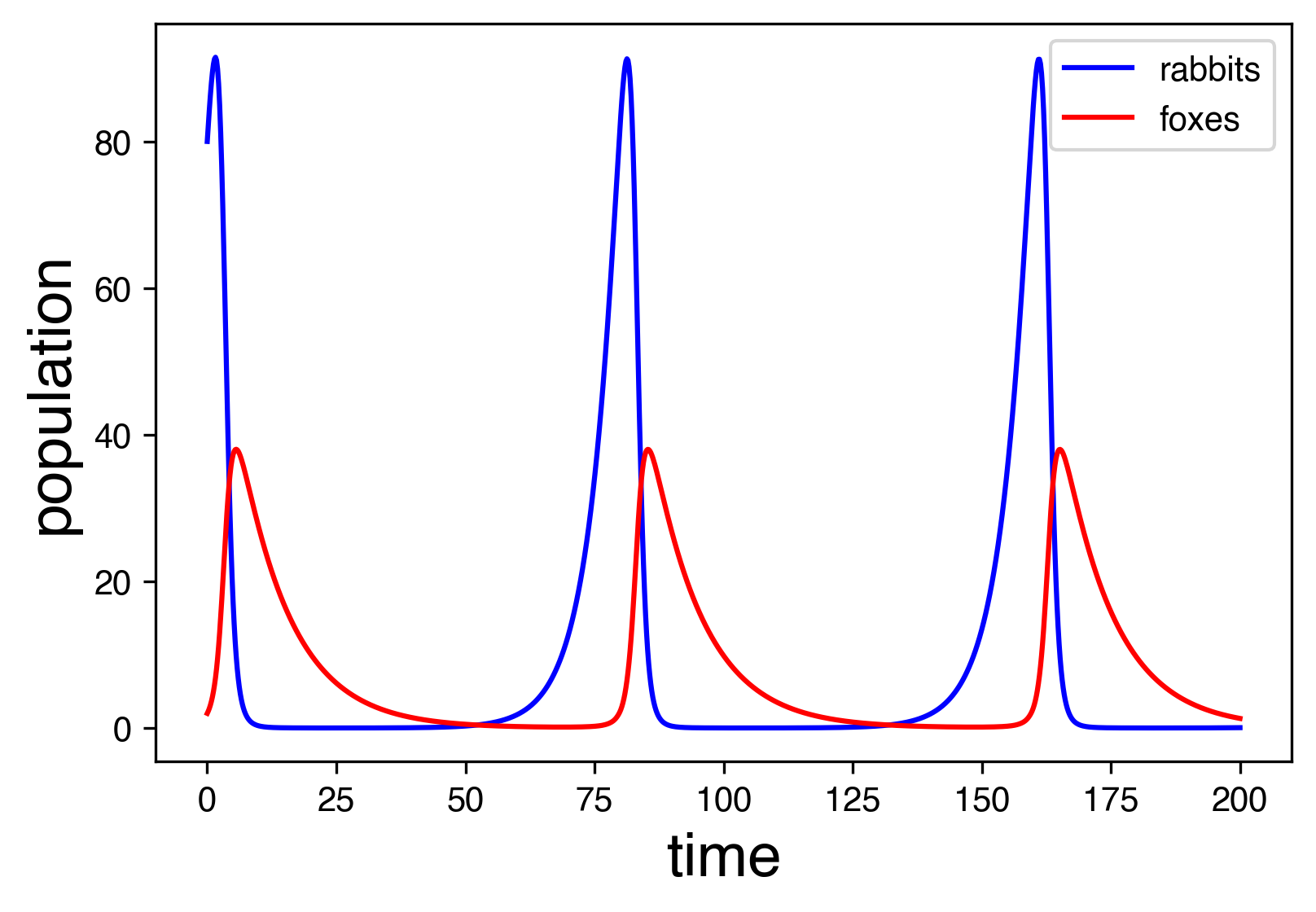
Figure 4:Periodic time evolution of the population of rabbits and foxes.
The solution is periodic. This can be illustrated better by plotting against . The animation below shows this (this kind of plot is called a phase plot).
Figure 5:Phase plot of the rabbit-fox prey-predator model. The red dot shows the population at different times. Note that the number of rabbits quickly increases when there are very few foxes. However, at some point the number of foxes also goes up and soon the start reducing the rabbits, while increasing in numbers themselves. That is not sustainable and when the number of rabbits is brought down substantially, also the number of foxes decreases, until both are almost extinct and the cycle repeats.
Wilberforce Oscillator
As a third example we look at the Wilberforce pendulum. This is a spring, suspended vertically, to which a weight is fixed at the free end. The weight can go up and down but also rotate in a horizontal plane. A sketch is given below.

Figure 6:Wilberforce pendulum.
Imagine that we pull a little down and let go. The spring will try to restore the position of the mass to the equilibrium position it was in prior to us pulling down. Consequently, will start oscillating in the vertical direction. However, something peculiar happens: the mass also starts to rotate (around the vertical axis). And also this rotation turns out to be a back and forth oscillation. But that is not all: the two oscillations are coupled: they feed each other. If the vertical oscillation is at a maximum amplitude, the rotational motion is almost zero and vice-versa.
A Wilbertforce pendulum made by first year physics students
The system can be modeled with simple means. We will just postulate them. Later on, we will see where the terms come from.
First, we note that the mass has kinetic energy, in two forms: due to the vertical motion () and due to the rotational motion (). Don’t worry about the exact meaning for now.
Second, the mass has potential energy. We will ignore gravity (we could for instance do the experiment in the International Space Station, ISS). A potential energy is associated with the vertical motion and is the spring energy: , with the vertical position of the mass with respect to the equilibrium position, which we took as . is the spring constant and represents the strength of the spring. We will come back to this later.
Then, we have potential energy associated with the rotation: . represent the rotation angle, where we have taken in the equilibrium position. is the torsional spring constant: it represents how strongly the spring tries to push back against rotation.
Finally, the vertical position and the rotation influence each other. That can be understood by realizing that if you shorten the spring, the spring material has to go somewhere. It cannot only change its vertical length as that would mean that the total length of the spring would reduce. But that would compress the spring material and that is not possible for solid material (unless you apply incredibly large forces). The spring just increases its number of windings a bit. But that implies rotation. Similarly, if we only rotate the spring, it will try to adjust its length. As a consequence, there is also a potential energy involved in the influencing of and of each other. It can be modeled as .
If we ignore friction, then we have a system that can be described in terms of energy:
From this, we can find ‘N2’, the equation of motion:
Don’t worry, if you don’t follow this. The point here is, that we have a coupled system of two oscillators. This can be solved numerically.
We could use a simple numerical scheme like we have employed in Chapter 3. In the figure below and are shown using such a simple numerical scheme.
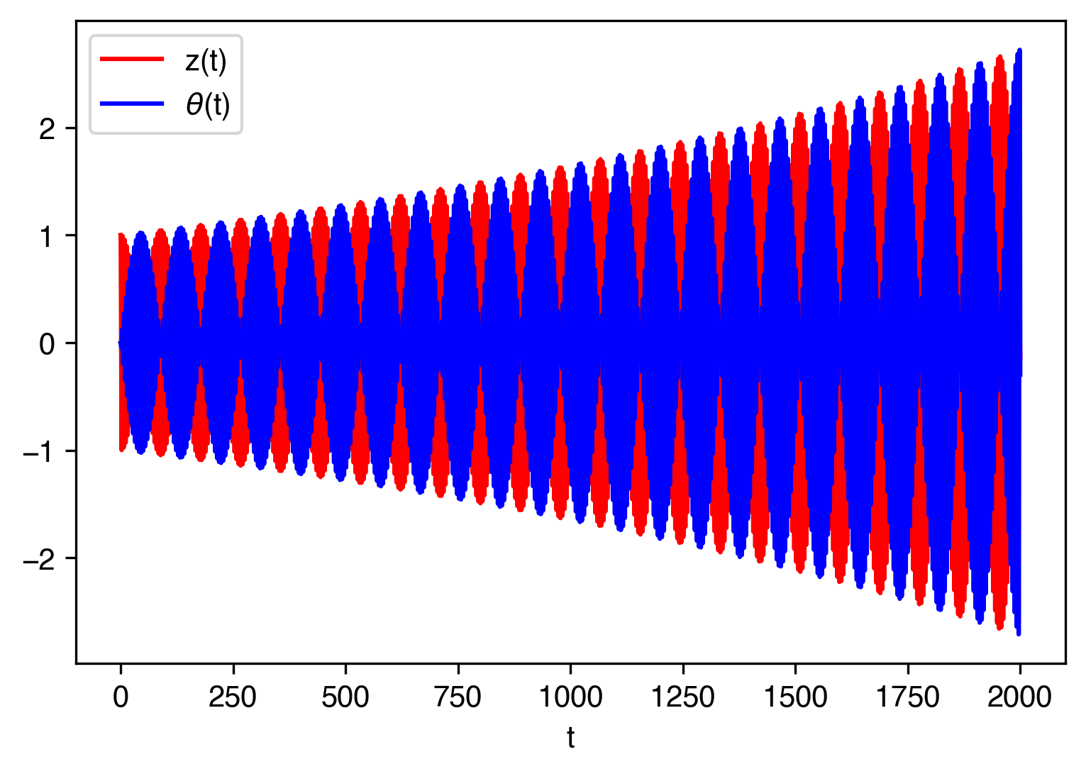
Figure 8:Numerical solution of the Wilberforce pendulum using a (too) simple numerical method.
We indeed see the oscillating motion and that the vertical oscillation changes over to rotation and back again.
But there is something really disturbing: the amplitude of our oscillation is increasing and it seems to do so for every cycle. That cannot be true: It violates energy conservation. What did we do wrong? Well, our numerical method is just not good enough. If we use again a higher order method, we obtain the results in the figure below.
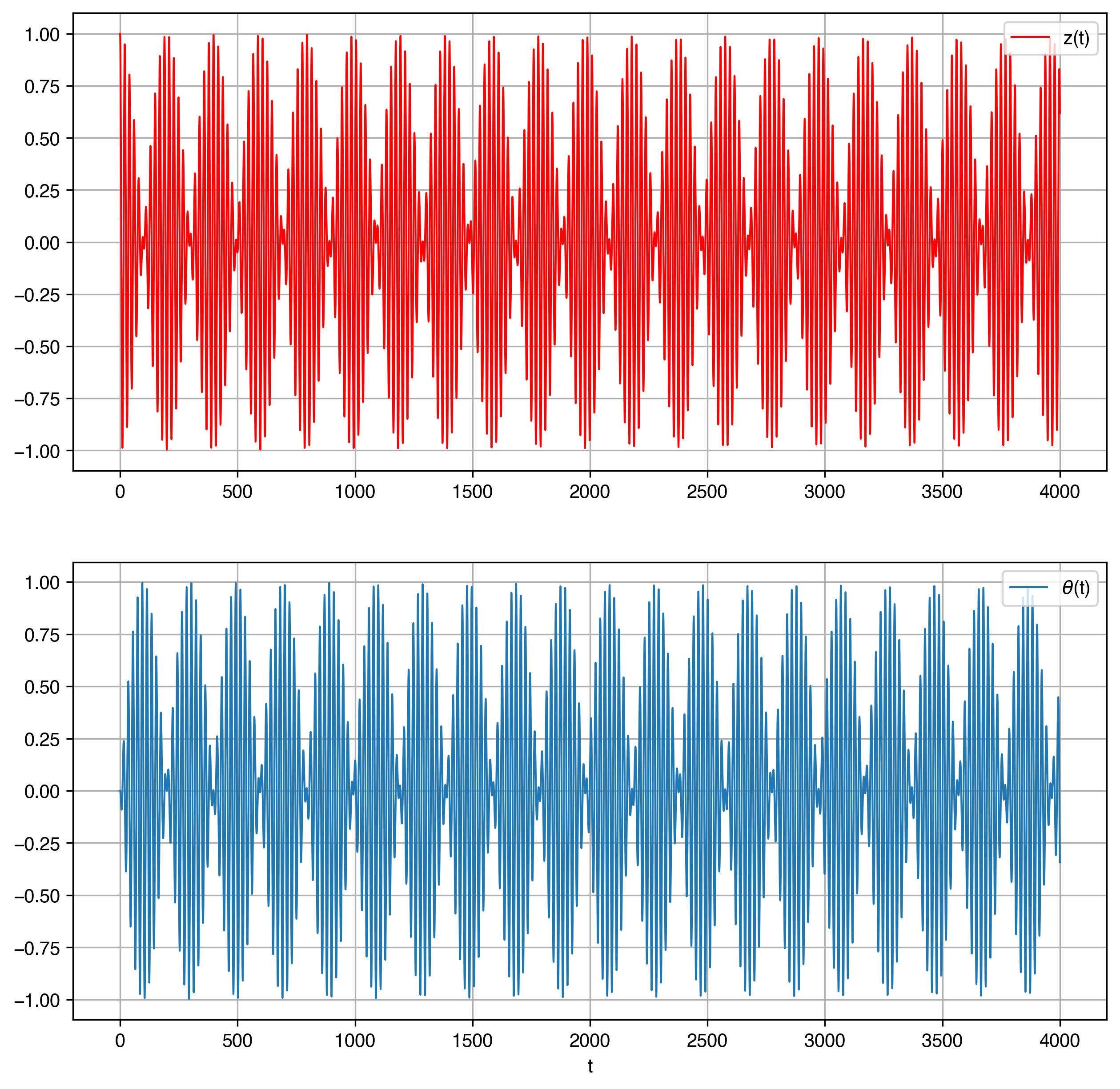
Figure 9:Numerical solution of the Wilberforce pendulum using a higher-order numerical method.
Now the amplitude of the oscillations stays nicely constant, obeying conservation of energy.
In the figure below a small animation can be seen: the marker in both graphs shows and at the same time instant.
Figure 10:Animation of the Wilberforce pendulum using a higher-order numerical method.
The Wilberforce pendulum is clearly periodic. Moreover, it is an oscillation as there is back and forth motion around an equilibrium.
But, it does give us a big warning: (numerical) solutions always have to be assessed against the features and principles of the problem at hand. In this case, our first numerical solution could not be right: it violated energy conservation. We were able, right from the start, to formulate the problem in terms of energy. Since we only had kinetic energy and potential energy we knew up front that the motion must be bounded!
That is why, we need a thorough understanding of physics. It is not sufficient to have the equations and put them in a ‘solver’. It is the job of a physicist to understand and assess models, outcomes, etc against the laws of physics. Hence, we will dive into oscillations, starting from the beginning.
Harmonic Oscillation - archetype: Mass-Spring
The archetype of an oscillation is the mass-spring system. It is the simplest version (simpler than the pendulum as we will see). And it can be recognized in many systems. We consider the following: a mass is attached to a spring. The other end of the spring is fixed. The mass can only move in one direction: the -direction. The spring has a natural or rest length . That is the length of the spring if no force is acting on it. If we pull the spring, it will exert a force that is proportional to the increase in length. Moreover, it is pointing in the direction opposite to the lengthening. In formula:
This is shown in the figure below.

Figure 11:Mass-spring system: archetype of a (harmonic) oscillation.
The response of the spring is to exert a force on proportional to its elongation (which may be negative, i.e. the spring is compressed). It is clearly a restoring force: no matter what we do pulling or pushing, the spring will always counteract.
It is not difficult to set up N2 for the mass-spring. There is only one force and the system is 1-dimensional. If we define the origin at the position of the mass when the spring is at its rest length, then - the elongation of the spring - becomes , the coordinate of the mass . Thus N2 reads as:
Or
To solve this, we need two initial condition. Let’s take . We need to find a function that upon differentiating twice it spits itself back but with an opposite sign. We do know two functions that do so: and . Thus, the general solution of the above equation is known.
Harmonic Oscillator:
If we insert the solution, we find
This is called the natural frequency of the oscillator. Note, that it does not depend on the initial conditions. No matter what, the mass will always oscillate with this frequency.
It does make sense that the frequency is inversely proportional to : we expect a heavy object will respond slow to a force. Similarly, if the spring is strong, that is has a high spring constant , it will move the mass around quickly.
If we substitute the initial condition, we can completely solve the motion of the mass:
A system is called a harmonic oscillator if and only if it obeys . You will find them in almost every branch of science and engineering. The reason why will become apparent in a moment.
Potential energy of a spring
In the above, we have formulated the mass-spring system in terms of Newton’s second law. We can, however, also cast it in the form of energy. The force of the spring is conservative. We can easily prove this by finding the associated potential energy: .
Since we need to find a function that satisfies . Let’s do it:
We have the freedom to decide ourselves where we want the potential energy to be zero. Note: is quadratic.
It does make sense, to set the minimum of the potential energy such that if the mass is at the equilibrium position, the potential energy is zero, that is - take :
Thus the mass-spring system can also be described by
So, an other way of stating what a harmonic oscillator is: it is a system that obeys the above energy equation.
Behavior around an equilibrium point and harmonic oscillators
Now we will go back to paragraph 5.5.1, where we discussed the Taylor series expansion of the function :
We will apply it to a potential energy of some system. We assume that the system has a stable equilibrium point at , that is
and .
Thus, we can expand the potential as follows:
If we plug this in, in the energy equation and cut off after the quadratic term, we find
or shortened by the abbreviation
Move the constant to the right hand side and change coordinate . This gives us:
The harmonic oscillator!!! No wonder we find harmonic oscillators ‘everywhere’. Any system that has a stable equilibrium point with a positive second derivative of its potential will start to oscillated as a harmonic one if we push it a little bit out of its equilibrium position. Doesn’t matter how exactly is. It doesn’t have to be quadratic in . But it will be pretty close to that, if we stay close enough to the equilibrium point. Hence, any small natural kick, any small amount noise will push a system out of its stable equilibrium point into an harmonic oscillating motion with a given, natural frequency given by .
Examples of Harmonic Oscillators
Torsion Pendulum
We take a straight metal wire. Suspend one end at the ceiling and attach a disc of radius and mass at the other end.

Figure 12:Torsion Pendulum.
The disk can rotate about a vertical axis. We call the rotation angle . The equilibrium position is . If we rotate the disc over a small angle, the wire will resist and apply a torque on the disc trying to rotate the disc back to its equilibrium position, for which the torque, obviously is zero.
For small angles, the torque is proportional to the rotation angle and -of course -working in the direction opposite of the rotated angle. We can set up an angular momentum equation and find that it reads as:
In this equation, is the moment of inertia of the disc and is the torsion constant of the wire. Don’t worry about the exact meaning of the terms in the equation. For now, we focus on the equation itself:
The torsion pendulum is a harmonic oscillator, , completely analogous to the archetype, mass-spring. Obviously, we thus can also write this in terms of energy:
with , the angular velocity.
L-C circuit
In Electronics alternating current (AC) circuits are building blocks of many complex systems. One of these is the L-C circuit, in which an inductor, , and a capacitor, , are in series coupled. See Figure 13.

Figure 13:L-C circuit.
We could charge the capacitor and then close the circuit. What would happen? The capacitor will try to discharge via the inductor. Hence a current, , starts flowing. In response, the inductor builds up a potential difference that is directly proportional to the rate of change of the current through the inductor.
Basic electronics shows that the voltage over the capacitor is coupled to the charge, , of the capacitor according to: . For the inductor we have: .
According to Kirchhoff’s laws the current through both elements must be the same: and the sum of the voltages across them must be equal to zero: . If we put everything together, we get - using :
As we see, this LC-circuit will start to oscillate. In the animation below the current through the circuit and the voltage across the inductor are shown for and .
Figure 16:Harmonic oscillation of an LC-circuit.
Musical Instruments
Musical instruments produce sound waves. In many cases they do that via vibrations of strings, like the guitar, the violin, harp or piano. The strings of these instruments are displaced out of their equilibrium position. Due to the tension in these strings, there is a restoring force that is proportional to the displacement. Consequently, the string will start to oscillate in an harmonic way.
Not only strings, but also beams will exhibit this behavior, well-known example: a tuning fork. We will come back to waves at the end of this chapter.
The pendulum
Another example of oscillatory motion is the pendulum. In it’s most simple form it is a point-mass , attached to a massless rod of length . The rod is fixed to a pivotal point that allows it to swing freely.

Figure 17:Sketch of a pendulum.
On the mass, gravity is acting vertically downwards. Also the rod exerts a force on the mass. This force is always parallel to the rod and points to the pivotal point. It is the response of the rod to the component of gravity parallel to the rod (the dark blue arrow in Figure 17). It is good to realize, that this force makes sure that the distance from to the pivotal point is always . In other words, this force is a consequence of the fixed length of the rod. It is the physics translation of the constraint: is constant.
N2 for the pendulum: Equation of motion via N2
We will set up Newton’s second Law for .
As stated above, the blue, parallel part of gravity is balanced by a tensional force in the rod. So, we don’t need to worry about motion of parallel to the rod. That leaves us with the direction perpendicular of the rod. In that direction only the red arrow works on .
In the other direction only the red, perpendicular component of gravity acts on . This component is equal to . The velocity component in this direction is . Thus we get:
Or rewritten
We do know from experience that the pendulum will swing back and forth in a periodic way. However, as we see from the above equation of motion: it is not a harmonic oscillator. The term with the sine prevents that.
But for small values of the angle , that is for small oscillations around the stable equilibrium , we can approximate the sinus via a Taylor series and write:
Thus within this approximation we can write for the equation of motion of the pendulum:
and that describes a harmonic oscillator.
We conclude that for small amplitudes of the oscillation, the pendulum is an harmonic oscillator and swings in a sine or cosine way back and forth. Moreover, the oscillation has a frequency
Further, note that under this assumption, the period of the pendulum does not depend on the amplitude of the oscillation. That was already noted by Galileo Galilei.
N2 for the pendulum: Equation of motion via Angular Momentum
Before we continue with the analysis of the pendulum, we will derive the equation of motion also via angular momentum considerations. On gravity exerts a torque: It has a magnitude and points into the screen. The angular momentum of is given by . This has magnitude and also points into the screen.
Thus N2 for angular momentum gives us:
Thus, angular momentum leads to the same equation of motion.
The Pendulum via energy conservation
Alternatively, we can also use energy conservation to derive the equation governing the motion of the pendulum. There are, as discussed above, two forces acting on . The first one is gravity, which is a conservative force with associated potential energy. We can write for this case , taking .
The second one is the force from the rod. But this one always acts perpendicular to the motion of . Hence, it does not do any work and, thus, we don’t need to worry about an associated potential.
We conclude that for the pendulum it holds that:
To solve this, we change from to . is, in terms of : , see Figure 18.

Figure 18:Potential energy of a pendulum.
Thus, our energy equation reads as:
or
Take the time-derivative and use and we get
And we have recovered the same equation of motion.
Pendulum for not so small angles
In the above we have frequently used the approximation for . What about the general case? Then we need to solve
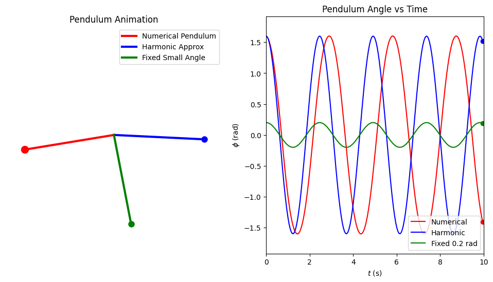
This equation is much more difficult to solve analytically and we will, therefore, use a numerical approach here. The animation below compares the motion of the pendulum numerically simulated to that of the pendulum when using the small amplitude approximation.
The animation shows: a green mass, that is the pendulum with a (fixed) small amplitude in the approximation . The blue one uses the same approximation even though is not small. Notice, that blue and green oscillate with exactly the same frequency. This is, of course, trivial as they obey the same harmonic oscillation equation and thus have the same frequency.
The red mass, on the other hand obeys the equation of motion of the pendulum leaving the term with . It is clear that the real pendulum (i.e. the red one) does not have the same frequency as the others. Moreover, its time trace (left part of the figure) is clearly not a true sinus.
Figure 19:Animation of the pendulum: red is the true pendulum, blue the small angle approximation applied to a large angle case and green the small angle approximation for a small angle.
In the widget below, you can vary the initial angle and observe that indeed for a small angle the red mass and the other two follow the same trajectory. But if you increase the initial angle, the red mass behaves differently: it oscillates slower and the time trace of angle as a function of time is no longer sinusoidal.
import numpy as np
import matplotlib.pyplot as plt
from matplotlib.animation import FuncAnimation
from IPython.display import HTML

# Parameters
L = 1.5         # Length pendulum (scaled)
g = 9.81        # Gravity (m/s^2)
phi0 = 1.6      # Initial angle (rad)
t_stop = 10     # Total time (s)
dt = 0.05       # Time step (s)

w0 = np.sqrt(g / L)

# Time array
t = np.arange(0, t_stop, dt)

# Numerical solution of pendulum using simple Euler method
phi_num = np.zeros_like(t)
w_num = np.zeros_like(t)
phi_num[0] = phi0
w_num[0] = 0
for i in range(1, len(t)):
    w_num[i] = w_num[i-1] - (g / L) * np.sin(phi_num[i-1]) * dt
    phi_num[i] = phi_num[i-1] + w_num[i] * dt

# Harmonic oscillator approx (small angle approx)
phi_harm = phi0 * np.cos(w0 * t)

# Green pendulum: fixed small angle 0.2 rad harmonic approx
phi_fixed = 0.2 * np.cos(w0 * t)

# Setup plot
fig, (ax1, ax2) = plt.subplots(1, 2, figsize=(12, 6))

# Left canvas: pendulum animation setup
ax1.set_xlim(-L*1.2, L*1.2)
ax1.set_ylim(-L*1.2, L*1.2)
ax1.set_aspect('equal')
ax1.set_title('Pendulum Animation')
ax1.axis('off')

rod_num, = ax1.plot([], [], 'r-', lw=3, label='Numerical Pendulum')
bob_num = ax1.plot([], [], 'ro', ms=10)[0]

rod_harm, = ax1.plot([], [], 'b-', lw=3, label='Harmonic Approx')
bob_harm = ax1.plot([], [], 'bo', ms=8)[0]

rod_fixed, = ax1.plot([], [], 'g-', lw=3, label='Fixed Small Angle')
bob_fixed = ax1.plot([], [], 'go', ms=8)[0]

ax1.legend(loc='upper right')

# Right canvas: angle vs time plots
ax2.set_xlim(0, t_stop)
ax2.set_ylim(-phi0 * 1.2, phi0 * 1.2)
ax2.set_title('Pendulum Angle vs Time')
ax2.set_xlabel('$t$ (s)')
ax2.set_ylabel('$\\phi$ (rad)')
line_num, = ax2.plot([], [], 'r-', label='Numerical')
line_harm, = ax2.plot([], [], 'b-', label='Harmonic')
line_fixed, = ax2.plot([], [], 'g-', label='Fixed 0.2 rad')
point_num, = ax2.plot([], [], 'ro')
point_harm, = ax2.plot([], [], 'bo')
point_fixed, = ax2.plot([], [], 'go')
ax2.legend()

def init():
    for artist in [rod_num, bob_num, rod_harm, bob_harm, rod_fixed, bob_fixed,
                   line_num, line_harm, line_fixed, point_num, point_harm, point_fixed]:
        artist.set_data([], [])
    return rod_num, bob_num, rod_harm, bob_harm, rod_fixed, bob_fixed, line_num, line_harm, line_fixed, point_num, point_harm, point_fixed

def update(frame):
    # Current angles
    phi_n = phi_num[frame]
    phi_h = phi_harm[frame]
    phi_f = phi_fixed[frame]

    # Coordinates for bobs (pendulum rods)
    x_num = L * np.sin(phi_n)
    y_num = -L * np.cos(phi_n)

    x_harm = L * np.sin(phi_h)
    y_harm = -L * np.cos(phi_h)

    x_fixed = L * np.sin(phi_f)
    y_fixed = -L * np.cos(phi_f)

    # Update pendulum rods and bobs
    rod_num.set_data([0, x_num], [0, y_num])
    bob_num.set_data([x_num], [y_num])

    rod_harm.set_data([0, x_harm], [0, y_harm])
    bob_harm.set_data([x_harm], [y_harm])

    rod_fixed.set_data([0, x_fixed], [0, y_fixed])
    bob_fixed.set_data([x_fixed], [y_fixed])

    # Update angle vs time lines (up to current frame)
    time_so_far = t[:frame+1]
    line_num.set_data(time_so_far, phi_num[:frame+1])
    line_harm.set_data(time_so_far, phi_harm[:frame+1])
    line_fixed.set_data(time_so_far, phi_fixed[:frame+1])

    # Update current points on the plots (wrap scalars in lists)
    point_num.set_data([t[frame]], [phi_num[frame]])
    point_harm.set_data([t[frame]], [phi_harm[frame]])
    point_fixed.set_data([t[frame]], [phi_fixed[frame]])

    return rod_num, bob_num, rod_harm, bob_harm, rod_fixed, bob_fixed, line_num, line_harm, line_fixed, point_num, point_harm, point_fixed

ani = FuncAnimation(fig, update, frames=len(t), init_func=init, blit=True, interval=50)
HTML(ani.to_jshtml())
The damped harmonic oscillator
In the above, no friction of any form has been considered. However, in many practical cases friction will be present. For moving objects friction frequently depends on the velocity: the higher the velocity, the higher the frictional force. We will here consider the simplest version: a friction force that is directly proportional to the velocity: with a positive constant. Thus, we need to add an additional force to our harmonic oscillator:
or bringing all terms to the left hand side:
To solve this equation, it is easier not to try to look directly for sinus and cosines, but use the complex notation.
The general solution of the (linearly) damped harmonic oscillator is:
We will investigate various cases.
In this case, the square root in is imaginary and we can write it as . This gives us for the two possibilities of
Both have the same real part: showing that both solutions are damped (with the same factor!). Moreover, the imaginary parts are equal, apart from the sign which we also had in the undamped case. We will write the imaginary part as (that is without the subscript 0 we used for the undamped case).
So, our solution reads as:
Conclusion: the damped oscillator oscillates with a smaller frequency than the undamped one and it amplitude decreases over time. The later is of course to be expected due to friction: sooner or later friction has dissipated all the kinetic & potential energy.
For this specific combination of we see that the frequency of the oscillation is 0. In other words, the systems does not perform oscillations. Furthermore, our two values of are now equal. Consequently the general solution that we presented is no longer complete (we now only have one integration constant, or only one independent function if you prefer.) We need a second one and that turns out to be of the form . You can verify that by substituting it in the equation of motion for the damped case.
Thus we have know:
Again, there is no imaginary part in , so no oscillations. But we do have two different values for and thus our original general solution is still valid:
Note that . So, both terms are decreasing to zero: the motion comes to a stop as .
Further, note that the first part (with ) has an exponent that is closer to zero than the one of the other part (with ). Thus the second part will decay faster and for sufficiently large , the solution behaves like .
In the figure below, an example of case 1 and case 3 is shown together with the solution of case 2. We see, that case 2 is the one that decays fastest: it has the highest damping coefficient in its exponent. This is called critical damping. If you need to dampen unwanted oscillations: make sure you tune your damping parameter b such that .
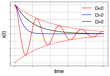
Figure 20:Different cases for the damped harmonic oscillator.
Evolution of the damping
Here we will have a quick look how the damping is evolving, that is we look at the root of the characteristic equation
and see how it evolves as a function of the damping in the complex plane.

Figure 21:Evolution of as a function of in the complex plane.
This gives quickly a qualitative view on the different regimes of the damping. The root is in general complex. We start by looking at the value for roots as a function of the damping
No damping: . The root is pure imaginary with two conjugate solutions on the imaginary axis. This gives pure oscillations.
Some damping . The root is complex, with real and imaginary part, the oscillation will damp out over time (shown in blue, underdamped regime).
. The roots collapse into one pure real root (critically damped), no oscillation.
Lots of damping . The root splits into two real roots, no oscillations (shown in yellow, overdamped regime).
The root walks over the shown graph from on the imaginary axis to over the blue and then yellow part of the graph. The yellow graph does not cross the imaginary axis.
From this plot you can directly see that the system is stable for , but unstable for without the need to check the frequency that the system is driven with (for driven with the resonance frequency results in an infinite amplitude - an instable system). How you can see that so quickly you will learn in the second year class Systems and Signals.
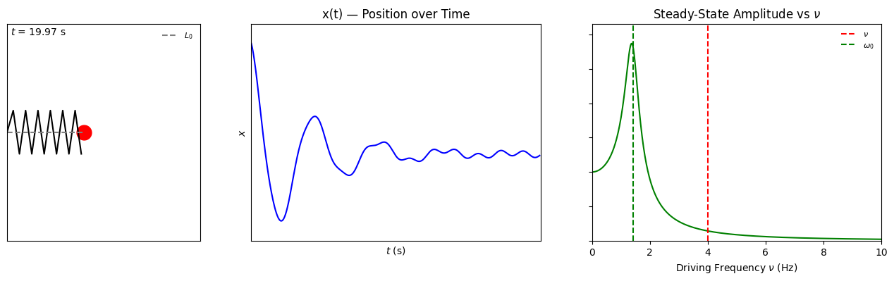
Driven Damped Harmonic Oscillator
Oscillators sometimes experience a driving force that can be periodic in itself. We will take here the case of a sinusoidal force with frequency . Once we understand this, forces consisting of more than one frequency (broader spectrum) can be understood using Fourier analysis (which you will learn about classes like Systems and Signals or Fourier Analysis in math). There you will also learn to treat this system in more detail analytically. Here we will stick to a simple driving force of the form .
This gives for the equation of motion:
with initial conditions: at the particle will have some position and some velocity .
The solution of the driven damped harmonic oscillator equation of motion for the case is:
With and determined by the initial conditions.
The two other parameters and are fixed. We will give only the expression for :
For , the second part, i.e., the term from the driving force , survives as the exponential decay will have damped the first term. The oscillation will have frequency of the driving force. As can be seen, the amplitude of the motion is for longer times .
If the driving frequency , the amplitude increases strongly. Especially for small damping, i.e., small , the amplitude will increase to high values. This phenomenon is called resonance:
Coupled Oscillators
In this course we mostly only consider one oscillator, but of course there could be many that are coupled in one way or another. Already Christiaan Huygens considered them.

Figure 22:Huygens experiment of weakly coupled pendula.
There are 2 pendula suspended from a common connection, which rests on two chairs. If you set the pendula in motion, they will be initially out of phase, i.e. the relative position of the pendula is different. But over time their motion synchronises! What has happend? Apparently the two pendula are connected, coupled, via the suspension and act on each other, they are not independent, but influence the motion of the other pendulum.
The following video of weakly coupled metronomes below shows a modern day version of this phenomena.
Here the pendula are coupled via the ground. This influence is called weak coupling. In this course we cannot treat this coupling mathematically, but in the second year course on Classical Mechanics you will learn to study systems like these.
Examples
Example of resonance: sound waves are exciting a glass. By changing the frequency of the sound waves to the resonance frequency, the glass starts oscillating with increasing amplitude until it finally breaks.
Driven harmonic oscillator with damping.
import numpy as np
import matplotlib.pyplot as plt
from matplotlib.animation import FuncAnimation
from matplotlib.gridspec import GridSpec
from IPython.display import HTML

# Parameters
m = 1
k = 2
b = 0.5
F0 = 20
nu = 4
l0 = 200
dx = 0.28 * l0

# Derived parameters
w0 = np.sqrt(k / m)
w = np.sqrt(w0**2 - (b / (2 * m))**2)
phi = np.arctan(-nu * b / m / (nu**2 - w0**2))
xmax = F0 / m / np.sqrt((nu**2 - w0**2)**2 + (b * nu / m)**2)

A = dx - xmax * np.cos(phi)
B = (1 / w) * (-A * b / (2 * m) + xmax * nu * np.sin(phi))

# Time setup
t_stop = 20
fps = 30
dt = 1 / fps
t_vals = np.arange(0, t_stop, dt)

# Position function
def position(t):
    transient = A * np.exp(-b / (2 * m) * t) * np.cos(w * t) + B * np.exp(-b / (2 * m) * t) * np.sin(w * t)
    steady = xmax * np.cos(nu * t - phi)
    return l0 + transient + steady

x_vals = position(t_vals)

# Steady-state amplitude over range of driving frequencies
nu_range = np.linspace(0, 10, 400)
xmax_range = F0 / m / np.sqrt((nu_range**2 - w0**2)**2 + (b * nu_range / m)**2)

# Set up figure and gridspec
fig = plt.figure(figsize=(16, 4))
gs = GridSpec(1, 3, width_ratios=[1, 1.5, 1.5])
ax_anim = fig.add_subplot(gs[0])
ax_xt = fig.add_subplot(gs[1])
ax_amp = fig.add_subplot(gs[2])

# --- Animation axis setup ---
ax_anim.set_xlim(0, 500)
ax_anim.set_ylim(-50, 50)
mass_dot, = ax_anim.plot([], [], 'ro', markersize=15)
spring_line, = ax_anim.plot([], [], 'k-', lw=1.5)
# Horizontal L0 line from wall to equilibrium position
l0_line, = ax_anim.plot([0, l0], [0, 0], linestyle='--', color='gray', label='$L_0$')
ax_anim.legend(loc='upper right', fontsize=8, frameon=False)
time_text = ax_anim.text(0.02, 0.95, '', transform=ax_anim.transAxes)
ax_anim.set_xticks([])
ax_anim.set_yticks([])

# --- x(t) axis setup ---
xt_line, = ax_xt.plot([], [], 'b-')
ax_xt.set_xlim(0, t_stop)
ax_xt.set_ylim(np.min(x_vals) - 10, np.max(x_vals) + 10)
ax_xt.set_xlabel("$t$ (s)")
ax_xt.set_ylabel("$x$")
ax_xt.set_title("x(t) — Position over Time")
ax_xt.set_xticks([])
ax_xt.set_yticks([])

# --- Steady-state amplitude axis setup ---
amp_line, = ax_amp.plot(nu_range, xmax_range, 'g-')
nu_line = ax_amp.axvline(nu, color='red', linestyle='--', label='$\\nu$')
w0_line = ax_amp.axvline(w0, color='green', linestyle='--', label='$\\omega_0$')
ax_amp.set_xlim(0, 10)
ax_amp.set_ylim(0, np.max(xmax_range) * 1.1)
ax_amp.set_xlabel("Driving Frequency $\\nu$ (Hz)")
ax_amp.set_title("Steady-State Amplitude vs $\\nu$")
ax_amp.legend(loc='upper right', fontsize=8, frameon=False)
ax_amp.set_yticklabels([])
# Function to draw spring as a zig-zag between 0 and x
def get_spring_coords(x, num_zigs=12, amplitude=10, end_offset=7):
    x_end = x - end_offset  # shorten to avoid overshooting the mass
    xs = np.linspace(0, x_end, num_zigs + 1)
    ys = np.zeros_like(xs)
    ys[1:-1:2] = amplitude
    ys[2::2] = -amplitude
    return xs, ys

def init():
    mass_dot.set_data([], [])
    spring_line.set_data([], [])
    time_text.set_text('')
    xt_line.set_data([], [])
    return mass_dot, spring_line, time_text, xt_line, nu_line, w0_line

def animate(i):
    x = x_vals[i]
    mass_dot.set_data([x], [0])

    # Update spring line with zig-zag
    xs, ys = get_spring_coords(x)
    spring_line.set_data(xs, ys)

    time_text.set_text(f"$t$ = {t_vals[i]:.2f} s")
    xt_line.set_data(t_vals[:i], x_vals[:i])
    return mass_dot, spring_line, time_text, xt_line, nu_line, w0_line

ani = FuncAnimation(fig, animate, frames=len(t_vals), init_func=init, blit=True, interval=1000*dt)

HTML(ani.to_jshtml())
Animation size has reached 21020492 bytes, exceeding the limit of 20971520.0. If you're sure you want a larger animation embedded, set the animation.embed_limit rc parameter to a larger value (in MB). This and further frames will be dropped.
1940: the Tacoma Narrows Bridge in the state Washington on the West coast of the USA is brought into resonance by the wind. See the movie clip for the end result.
Breaking a HDD hard disk with a song of Janet Jackson
Read here about this truly amazing piece of applied physics on a blog of Microsoft developer Raimond Chen.The blue sky: Rayleigh scattering (adapted from Mudde (2008)).
Light from the sun (and stars) will have to travel through the atmosphere before reaching the ground level. On its way it will be subject to absorption and scattering.
When you look on a clear day into the sky its color is blue, everybody knows that. But few people know why. The reason is found in the scattering properties of the molecules: the probability of light being scattered by an air molecule is proportional to the wave length of the light to the power -4, or rephrased: proportional to ( the frequency of the light, the theory of molecular scattering was given first given by Lord Rayleigh). Thus, blue light of a wavelength of 450nm is compared to red light ( = 650nm) times more likely to be scattered. Consequently, the blue end from the (white) sun light has a reduced probability to reach our eye directly in comparison with the red end. And thus most of the scattered light that reaches us is blue: the sky is blue.
We will look at scattering of light by considering a simple molecule made of a fixed nucleus with one electron orbiting it. The equation of motion of the electron can be written as that of a harmonic oscillator, with eigen frequency :

Figure 23:Simple model of electron-light scattering.
When light passes the electron, the electron feels a force since light is an electro-magnetic wave. The electric field is the dominating force. For light of wave length , i.e. angular frequency , the electric field can be written as . Such a field will produce a force on the electron, modifying its equation of motion to:
We recognize this as the forced harmonic oscillator with solution
The important part is the last one: the extra motion cause by the passing electric field. This causes an additional acceleration of the electron: .
The electron in its original orbit does not radiate. However, due to the extra acceleration the electron starts radiating. It sends out an electromagnetic field with the wave length of the incoming light and an intensity proportional to the square of the acceleration, , i.e.
As the eigen frequency of the electrons in oxygen and nitrogen is much higher than the frequency of the incoming light we have that this is basically proportional to . As this radiation by the electron obviously feeds on the incoming light, we find that the scattering of the light is proportional to the frequency of the incoming light to the power 4.
Second-harmonic generation
Of course the harmonic potential is only a first order approximation around an equilibrium. An example, for a non-linear force or anharmonic potential effect, is the generation of second-harmonic generation. If you shine high intensity light onto the electrons of a molecule, they are pushed out of equilibrium further and if the governing potential is anharmonic, the electric field response will not only include the incoming frequency but also higher harmonics , but with much lower intensity. That the emitted frequencies are occurring in integer multiple of the incident frequency can be understood either from quantization of light into photons (and the conservation of energy) or from Fourier analysis of the periodic motion of the electron.Erasmus Bridge & singing cables.
The bridge in Rotterdam, but also others, suffer from long cables that the wind can put into resonance. Their motion then generates acoustic waves in the audible spectrum. Listen here to the sound of the cables starting from 1:00 on the website for singing bridges!
Waves and oscillations
In the previous sections, we talked about oscillations of individual particles. Oscillations can also occur in a more collective mode. And there are plenty of examples: take for instance a violin or piano string. It is in essence an elastic string suspended between two fixed points. The string is under tension, that is: its natural length is (slightly) less than the distance between the two end points. As a consequence, equilibrium position of the string is a straight line and when brought out of equilibrium there is a net restoring force much like for the mass-spring system.
However, there are at least two important differences: (1) the restoring force is the net result from pulling on a small part of the string by its neighbor parts; (2) the entire string can oscillate in a direction perpendicular to the equilibrium position of the string, making the problem multi-dimensional.
We will give here an intuitive derivation of the equation of motion. Don’t worry if you don’t grasp it fully. This will come back in your studies further down the line.
In the figure below, a part of the string is drawn with special attention to a small part (the red line). On this small part the tension from the left and right side is pulling on the red part. This is visualized by the two blue arrows. In the inset, this is drawn at a larger scale. The two blue arrows are equal in magnitude () as the tension in the string is the same everywhere. But the direction in which the two blue forces are pulling is slightly different as the string is curved.

Figure 24:Forces on a small part of a string; inset shows an exaggeration of the vertical components of the forces.
If we call the angle of the blue forces with the -axis , then . This makes that a net force is action on the small red piece. And according to Newton’s second Law, the small red mass must accelerate.
Let’s set up N2 for the red piece. The problem is 2-dimensional, so we set up N2 for the and -direction:
Next, we simplify by only looking at situations where the angle and are small. The we can approximate the and terms: if then and and we can write
Thus: for the direction we don’t need to worry, nothing interesting happening there.
For the -direction we face that we have too many unknowns. We need relations between and . We are going to use again that but know to make it seemingly more complex.
If then . And we are going to replace by . Is that smart??? Now we get trigonometry back in the equation!! Don’t worry. We use the in another way. It is also the direction of the tangent to the curve the spring is making at the point where we are looking. In formula:
And this is the coupling between angles and coordinates that we have been looking for.
We are going to plug this in in N2 for the -direction. But before doing so: the left position of the red piece is at position . So instead of label ‘1’ we will use subscript . Similarly, the right end of the red piece is at . Thus we can write
It looks still pretty messy but we are almost there. The mass of the red piece obviously scales with its length. So if we introduce as the mass of the string per unit length, we can write for the mass of the red piece: . Our equation can now be written as
We recognize on the right hand side the second derivative of with respect to . Whereas on the left hand we see differentiating with respect to .
To make clear that we mean on the left hand side we mean: take the derivative only with respect to time we use instead of . Similarly on the right hand instead of . And we get our final result replacing by
This equation is called the wave equation and you will find it back in many branches of science and engineering. To solve it, you need advance calculus and that will certainly come in future courses. Here we will look at some global aspects of the equation.
units of . Thus is a kind of velocity, at least based on its dimension.
if is such that it only depends on , that is then no matter what as function is, it is always a solution to the wave equation.
This is straightforward to prove: given then call
Note the meaning of : differentiate as if is a constant, not depending on .
We can differentiate this once more:
Subsequently we look at :
If we now substitute these two results in the wave equation we see:
And we see that our choice for automatically obeys the wave equation.
From the above we also learn that if the string has a certain ‘amplitude’ at position on time a little later this same amplitude will show up at a position a bit further along the string. Argument: given and then at the amplitude of the string is and a little later, at we can look at position : there is
This actually means, that a traveling wave can be present in the string. We now this from our childhood when we probably all have been playing with a long rope making waves in it by quickly moving one end up and down.
The wave equation has as constant . We have identified this as a velocity and we now understand that it is the velocity with which a wave travels. But since the equation contains the square of the velocity, we conclude that if we have a solution with , then also a solution with holds. In other words: waves can travel in 2 directions and they do so with the same speed (in magnitude).
In the figure below, a wave is shown that starts as seemingly one hump. But it actually is two traveling waves on a rope.
Moreover, the rope has a fixed end at the left and a free one at the right. Notice the difference in reflection of the waves at both ends.
Figure 25:Forces on a small part of a string; inset shows an exaggeration of the vertical components of the forces.
Wave characteristics
Waves are omnipresent. We find them in musical instruments e.g. the violin but also in flutes where the wave is directly in the air in the instrument. We have them in water and air: waves on the oceans, waves when we speak. There are waves in solid materials for instance after an earthquake. We use waves in telecommunication.
Why are waves so generally found? They are the analogue of the harmonic oscillator. And thus, many systems in that are brought a bit out of equilibrium will try to go back to equilibrium, over shoot it and end up in a wavy motion.
Wave Length
Waves are often sinusoidal and if not, via Fourier Analysis they can be decomposed of a set of sinusoidal waves that built together the pattern we observe.
A sinusoidal wave is of the form
with its frequency (and thus its angular frequency).
As we have seen above, in general the wave is also a function of position:
How can we connect these two forms? First, we need to realize that the last equation has a dimensional issue: what is the sinus of say 7 meter? In other words, the argument of the sin-function should be dimensionless. So we write is in a different form, introducing the frequency in it:
This seems unnecessary complicated. But it is not! The factor has dimension 1 over length. If we call it we can write
Interpretation: for a fixed value of the wave is periodic in space with period . This is what we already know: the wave has a wave length .
On the other hand: for a fixed position the point at oscillates with a frequency and thus has a period . Note that and are coupled to each other:
Standing waves versus traveling waves
If we look at the motion of the string on a violin closely, we will not see traveling waves running from one side of the string to the other. Instead, we see all parts of the string moving up and down collectively: they have formed a standing wave. that is a wave that does not travel, but has a fixed, stationary shape whose amplitude various with time.
For a string with two ends fixed like on a piano or violin, the string can only show standing waves that ‘fit’. These standing waves are sinusoidal and their wave length should be such that the beginning and end of the string don’t oscillate. In the figure below four possibilities are shown.
Standing waves in a string.
We see that there is a simple relation between the length of the string, and the possible wave length, of the standing waves:
Further we see that the smaller the wavelength, the faster the oscillation. This is due to the relation that still holds: .
The traveling waves had as mathematical form . The standing waves take forms like . You will learn much more about this in e.g. Fourier Analysis classes.
Water waves and Sound waves
It is not necessary that a wave is caused by a tension in the material that tries to restore the equilibrium position. The restoring force can be of a different nature. A well know example is the water waves that we see on lakes and seas. Here gravity is the restoring force: it tries to pull a crest down and push a through up. The water inertia causes overshoot resulting in oscillations, that we call waves. In dealing with waves, we usually don’t use the frequency , but instead the angular velocity . Similarly, frequently the wave length is replaced by the wavenumber . Note that these two quantities are also related to each other by the speed of the waves: .
For water waves (with large wave length) the angular momentum and the wave number are coupled to the depth, , of the water:
From this we learn that waves on deep water travel much faster than on shallow water. This can be seen on our shores: the waves coming from the open sea are slowed down when the approach our beaches. But behind them the fast ones still come in. As a consequence, the wave gets squeezed in length and thus must get higher. This can be extreme with dramatic consequences: the Tsunami. The wave of the Tsunami is formed out in the open, where the sea is very deep. Here it travels at a very high speed which also means that it is a long wave. The Tsunami waves can travel at velocities of 200m/s and have wave length of hundreds of kilometers. However at full sea their amplitude is in the centimeter, decimeter range. A ship at full sea will hardly notice the passing Tsunami wave. But when the approach the shore, the front of the wave is slowed down to tens of m/s. As the back is still coming in at full speed the wave amplitude has to increase. And thus a huge wave in terms of amplitude storms towards the shore. A wall of water is seen coming, crushing everything in its way.
Sound waves are another type of waves that occur frequently. They can exist in solids, liquids and gasses. In contrast to the waves we have discussed so far, the amplitude is not perpendicular to the direction of traveling. It is what we call a longitudinal wave that oscillates in the same direction as it moves. The other waves are called transversal waves.
For sound waves it is the pressure that is the restoring force. The ‘crest’ is compressed material, the ‘through’ is an expansion part. Newton was intrigued by sound waves and provided a theory for them. He found that the speed of sound in air, according to his theory, was about 290 m/s. In reality it is some 340 m/s. Newton was well aware of the mismatch. But he couldn’t find a good explanation. It took another 100 years for Pierre Laplace corrected Newton’s work and arrived at the correct answer. Newton did not know that sound is connected to adiabatic compression. He couldn’t as the entire concept was not know. Laplace realized that Newton basically had made an isothermal solution and corrected this.
On Taylor expansion
import numpy as np
import matplotlib.pyplot as plt
import ipywidgets as widgets
from ipywidgets import interact
import math

x = np.linspace(0,2*np.pi,1000)
y = np.sin(x)


def taylor_series(x, n):
    ts = np.zeros_like(x)
    for k in range(int(n)):
        ts += ((-1)**k * x**(2*k+1)) / math.factorial(2*k+1)
    return ts

def update(n):
    plt.clf()
    plt.figure()

    plt.plot(x,y,'k.')
    plt.plot(x,taylor_series(x,n))

    plt.ylim(-5,5)
    plt.show()

# Use FloatSlider for smooth interaction
interact(update, n=widgets.FloatSlider(min=1, max=20, step=1, value=4))- Mudde, R. F. (2008). Surrounded by Physics. VSSD.
- Pols, F. (2021). The sound of music: determining Young’s modulus using a guitar string. Physics Education, 56(3), 035027. 10.1088/1361-6552/abef07