Jupyter Book 2 (JB2) supports both Markdown files and Jupyter Notebooks as content sources.
Markdown
Markdown is a simple markup language: plain text that is formatted with small pieces of ‘code’. This allows you to create rich, interactive books that combine text, code, and visualizations. This text can then be quickly exported to various other formats such as PDF, Word, HTML, etc.
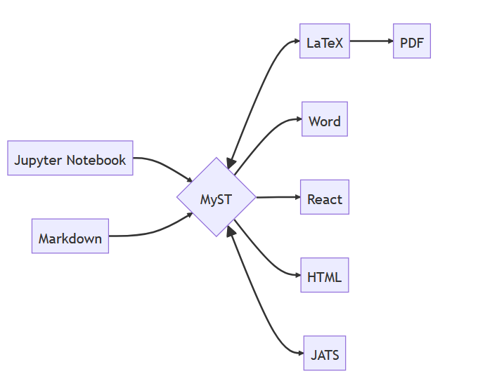
Documents made in MyST Markdown can be converted to many different formats. These can be saved as JSON, or rendered to a website (like this one!) or any number of formats including PDF & LaTeX, Word, React, or JATS. Picture taken from the MYST documentation [1].
See below for an example of the Markdown language and how it is rendered in JB2.
This is a heading
This is a paragraph with bold and italic text.
This is a list item
Another list item
# This is a heading
This is a paragraph with **bold** and *italic* text.
- This is a list item
- Another list item
```{warning} raw HTML
You can also include raw HTML in your Markdown files, but this will not be rendered in the PDF output.
```
In the next chapter we cover most of the basic Markdown syntax you will need to create your own content.
Jupyter Notebooks
Jupyter Notebooks are interactive documents that combine live code, equations, visualizations, and narrative text made with Markdown. They are widely used for data analysis, scientific research, and teaching, allowing users to run code in a step-by-step manner and see immediate results.
JB2 allows to include Jupyter Notebooks directly in your book, making it easy to share interactive content with your readers. It also allows to run code cells and display the output directly in the book. Check the output below by first clicking the ON-button at the top right of this page. This loads the server. Once it is ready, you can run the code cell below by clicking the play button.
print("Hello, World!")Cell Tags and Hiding Input
Cell tags in Jupyter Notebooks are metadata labels that you can assign to individual cells. They are useful for customizing the behavior of cells, such as hiding code input.
To hide the input of a code cell (so only the output is visible), you can add a tag like hide_input to that cell. JB2 recognizes this tag and will hide the code input when rendering or exporting the notebook.
Source
import numpy as np
import matplotlib.pyplot as plt
from matplotlib.patches import Rectangle
from matplotlib.transforms import Affine2D
from ipywidgets import interact
import ipywidgets as widgets

# Constants
start = [0, 0]

L = 2
m = 10 #kg
g = 9.81 #kgm/s^2
t = np.linspace(0,5,100)

def Fw(theta,mu):
    return mu*m*g*np.cos(theta)

def Fzx(theta):
    return m*g*np.sin(theta)

def update(theta,mu):
    # Compute arrow end coordinates
    end = np.array([L * np.cos(theta), L * np.sin(theta)])

    # Clear figure
    plt.clf()
    fig, axs = plt.subplots(1,2, figsize=(10, 5), gridspec_kw={'wspace': 0.4})

    # first plot showing angle and box
    ax = axs[0]
    ax.set_xlim(0, 2)
    ax.set_ylim(0, 2)
    ax.set_aspect('equal')
    ax.grid(True)

    if Fw(theta,mu)>Fzx(theta):
        ax.text(1.5, 1.5, 'Stable', fontsize=12)
    else:
        ax.text(1.5, 1.5, 'Sliding', fontsize=12)
    # Draw arrow
    ax.arrow(start[0], start[1], end[0], end[1],
             head_width=0, head_length=0, fc='black', ec='black')

    # Box properties
    box_width = 0.4
    box_height = 0.2

    # Create unrotated rectangle at (0,0)
    rect = Rectangle((-box_width / 2, 0 ),
                     box_width, box_height,
                     linewidth=1, edgecolor='red', facecolor='lightgray')

    # Compute arrow end coordinates
    end = start + np.array([L * np.cos(theta), L * np.sin(theta)])

    # Compute midpoint of arrow
    mid = start + np.array([L/2 * np.cos(theta), L/2 * np.sin(theta)])

    # Transformation: rotate around origin, then translate to arrow tip
    trans = (Affine2D()
             .rotate(theta)
             .translate(mid[0], mid[1]) + ax.transData)

    rect.set_transform(trans)
    ax.add_patch(rect)

    # second plot showing motion with and without friction
    ax2 = axs[1]

    ax2.set_xlabel('$t$(s)')
    ax2.set_ylabel('$s$(m)')


    ax2.plot(t,1/2*g*np.sin(theta)*t**2,'k-',label='without friction')

    if Fw(theta,mu)>Fzx(theta):
        ax2.plot(t,np.zeros(len(t)),'r-',label='with friction')
    else:
        ax2.plot(t,1/2*g*(np.sin(theta)-mu*np.cos(theta))*t**2,'r-',label='with friction')


    ax2.set_ylim(0,120)
    ax2.legend()


    plt.show()

# Use FloatSlider for smooth interaction
interact(update, theta=widgets.FloatSlider(min=0, max=np.pi/2, step=np.pi/16, value=np.pi/4),
         mu=widgets.FloatSlider(min=0, max=1, step=0.05, value=1))
To add a tag:
Select the cell.
Open the “View” menu and enable the “Cell Toolbar” → “Tags”.
Add the tag
hide_input(or another tag recognized by your toolchain).
This feature is especially useful for creating clean, reader-friendly notebooks where you want to focus on results rather than code details, see below.
The code above provides a semi-interactive simulation: you are able to change two parameters but cannot control/adapt the code itself. This will be available in the near feature.