As the years progressed, Classical Mechanics developed further and further. So, in the first half of the nineteenths century it felt like classical mechanics was an all encompassing theory and that physics would become a discipline of working out problems based on a well-established, complete theory. But that wasn’t going to be the case at all. Around 1850-1860 several cracks in the theory started to become visible. And they were fundamental!
Rutherford & the atom
Atomic theory
The idea that matter is made of atoms is old. However, the notion of atoms as we have now is relatively young.
In the ancient Greek world, it was as early as the fifth century B.C. that Leucippus and later one of his pupils Democritus proposed that the world (matter), is made up of tiny, indivisible particles. These particles were called atoms, derived from the Greek word ‘atomos’, which means uncuttable. These particles would float in a vacuum, that was called void by Democritus. We currently have a view that is remarkably close, but at the same time quite different from these first ideas.
In ancient India even earlier (records go back to the eighth’ century B.C.) philosophers like Uddalaka Aruni talk about matter being made up of tiny particles. They did not use terms like atoms, but instead referred to the ‘building blocks’ of matter as ‘kana’ which means particles. In the Islamic world, atomic theories were developed in e.g. the Asharite school by Al Ghazali (1058-1111). In his thinking, atoms are the only material things that live forever. Everything else, any event or interaction is due to God’s intervention.
Although these early thoughts point at atoms as the underlying elements of matter and as such resemble our current understanding of matter, they also differ quite a bit. The early ideas are based on philosophy and the notion that matter is either a continuum that can always be cut in smaller parts that still maintain all characteristics or that at some point a further splitting in smaller pieces is no longer possible with at least losing some of the characteristics.
In more recent history, the notion of atoms as elementary building blocks is guided by experiments. The English physicist and chemist John Dalton (1766-1844) did ground breaking work. He noticed that water, when decomposed, always resulted in the same elements: hydrogen and oxygen. Moreover, the relative weights of these two was always the same. Furthermore, he came to the conclusion that there is a unique atom for each element. More chemists noted that many substances were made of the elements in very specific ratios. In our modern view we would say: water is formed in a 1 to 2 ratio of oxygen and hydrogen, never in 1 to 2.1 or any other non-integer number.
Although the evidence from chemistry was clear, the notion of atoms as the building blocks remained controversial. The laws of definite proportion (e.g. water is decomposed in a fixed ratio in hydrogen and oxygen) were generally accepted, but the hypothesis that everything was made of atoms was not. As a consequence, the work of Ludwig Boltzmann (1844-1906) on statistical thermodynamics that is entirely based on an atomic (or molecular) view was not accepted during Boltzmann’s life.
In the second half of the nineteenth century William Thomson (1824-1907) - later Lord Kelvin - proposed the so-called vortex theory of the atom. Based on the discoveries by chemists of only a few different atoms that made up the rest of matter, Thomson proposed that atoms are stable vortices, not in an ordinary fluid like water, but in the omni-present luminiferous aether (ether).
Stable vortices have the shape of rings with no beginning or end. In air they are easily made and made visible with smoke and are indeed surprisingly stable. According to the vortex theory, atoms are vortices in aether. The simplest one is a single ring, which was hydrogen. More complicated forms, called knots represented the other elements.
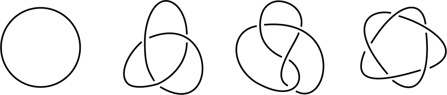
Figure 1:Various vortex knots, each represents another element. From Wikimedia Commons, public domain.
At the end of the nineteenth century, in 1897, Joseph John Thomson discovered the electron. It allowed him to further refine the scientific model of the atom and ended the vortex theory. In Thomson’s view, an atom has internal structure: the electrons are moving in it. As electrons have a negative charge and atoms are neutral, there must be a balancing positive charge in an atom as well. Thomson had no idea what that would be. He figured that the positive charge was everywhere in the atom (that he thought of as being a sphere), with the electrons moving inside that sphere as tiny particles. From this picture, the Thomson model got its name: the plum pudding model, although it is a bit misleading as the idea was that the positively charged sphere was more a liquid in which the electrons ‘float’ than a solid.
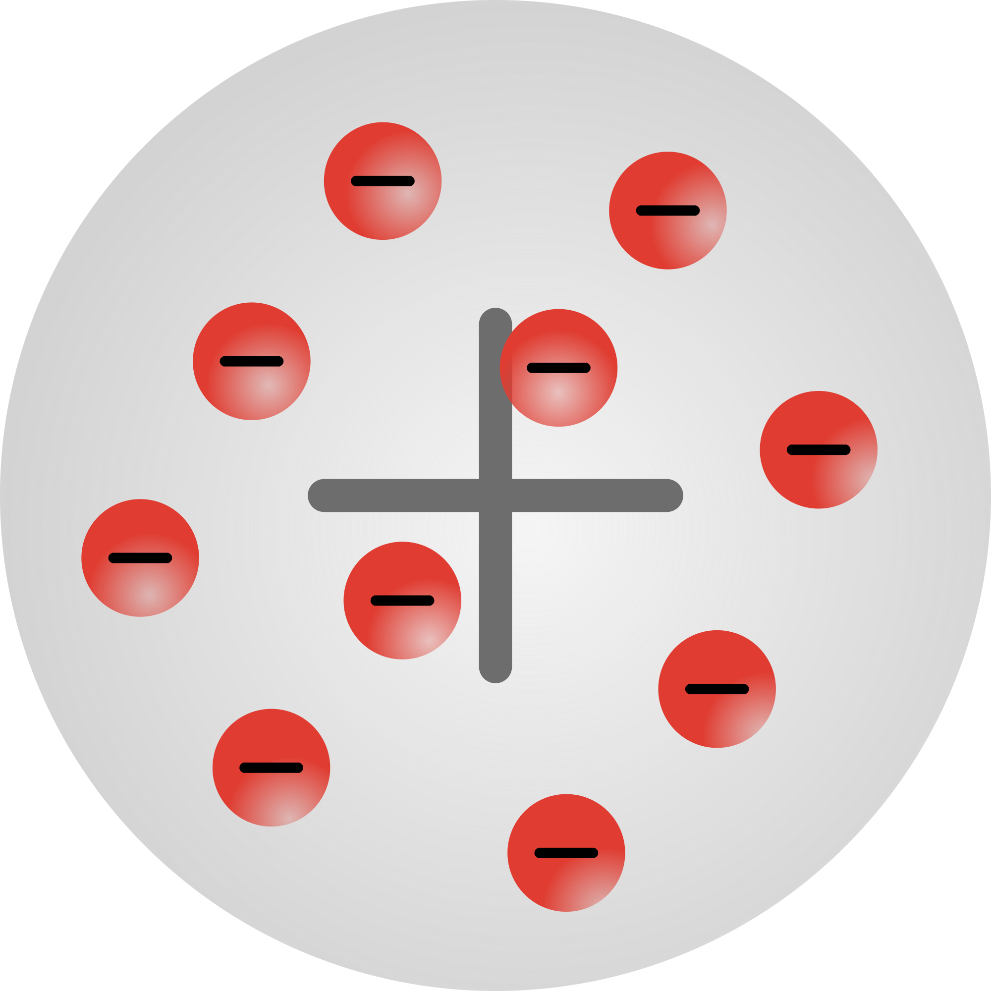
Figure 3:Plum pudding model according to Joseph Thomson. From Wikimedia Commons, public domain.
The model did not hold very long as we will see in the next paragraph. Nevertheless, it marks the start of physicist becoming really interested in an atom theory.
Rutherford’s scattering experiment
The plum pudding model was abandoned in 1911. That year Ernest Rutherford (1871-1937), a former student of Joseph Thomson, performed a ground-breaking experiment. Rutherford had been working on the newly discovered radio-activity of certain elements. He discovered that there were two types of radiation that were different from X-rays. He called them ‘alpha’ () and ‘beta’ () rays. Later he proved that ‘alpha’ rays consist of He-nuclei. Rutherford, in cooperation with Frederick Soddy, was the first one to prove Marie Curie’s conjecture that radioactivity was an atomic phenomenon, which could lead to changes in the atom itself, from one element to another. This idea thus countered the prior idea that an atom was seen as the ultimate, indestructible form of matter: atoms could not change from one form (element) to another.
Rutherford, in cooperation with Hans Geiger (one of the inventors of what we now call the Geiger counter) and Ernest Masden, built an apparatus that could count the -particles. Moreover, he showed that the -particles were He-nuclei with a positive charge of . In 1917, he showed that Nitrogen could become Oxygen by bombarding it with the -particles. This was the first time that someone succeeded in artificially changing one element into another.
Scattering at a gold foil
As mentioned, Rutherford is responsible for overthrowing the plum pudding model and replacing it by our modern view: an atom is made of a tiny, positively charged nucleus with the electrons orbiting around it.
The start of this paradigm-shift was formed by Rutherford’s observation that some of the -particles were deflected by a thin metal sheet in front of his -counter. This puzzled him as the plum pudding model could not explain this: when using that model the particles were either colliding with only small deviations or passing straight. Rutherford, Geiger and Marsden thus set up an experiment in which they led the -particles scatter at a very thin gold foil to investigate further.
In the experiment, the source would emit -particles through a small diaphragm onto the gold foil. The diaphragm made sure that all -particles were traveling on the same line. After moving through the gold foil, the particles could be detected by looking via a microscope at the tiny light flashes an -particle caused when hitting the detection screen. The microscope and detection screen could be placed under an angle with the original trajectory of the -particles. By measuring at all possible angles, the scattering of the -particles by the gold foil could be completely mapped and quantified.
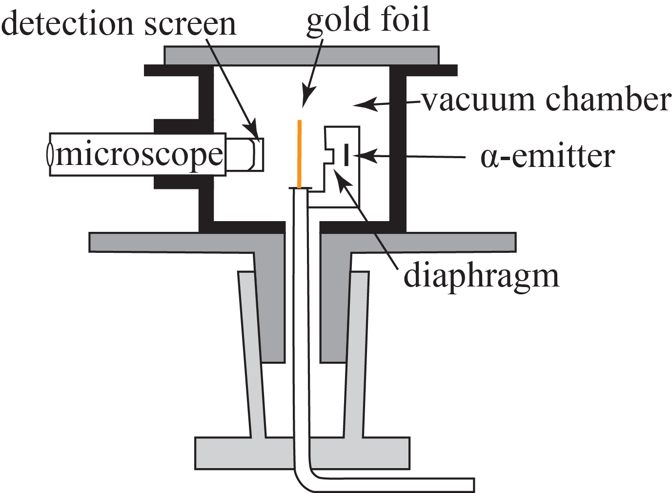
Figure 6:Experimental setup of -scattering at a gold foil.
The story goes, that Rutherford’s students would, together with Geiger, do the measurements as an assignment of their studies. The principle is simple: set the microscope under a known angle and, for a given period in time, count the number of hits. Repeat this for the next angle of the microscope. Obviously, the first measurements were all done on the side of the foil opposite to the -emitter. One was expecting small deviations from the undisturbed trajectory.
When the experiments were basically done, so the story goes, still a student was left over that also needed an assignment. One of Rutherford’s assistant suggested that this student would then measure with the microscope at the same side of the foil as the -emitter. They did not expect anything to see, but they needed an assignment for this student. Whether the story of the student assignments is true or not, fact is that the team found also hits on the detector for angles of about 180°. That is, some -particles seemed to bounce back from the foil!
There is no way that the plum pudding model could explain this. The argumentation to show that, goes as follows.
The size of the atoms of gold is known: they are on the order of .
This value can be found from the density of gold, the mass of a gold atom and the mass and volume of the gold foil (or any other amount of gold). By treating the atoms as small spheres that are stacked back to back, the size of the atom is easily found.An -particle has a charge of and is deflected by a gold atom due to the charge of the gold atom. As gold has number 79 in the periodic table, we know that the charge of a gold atom is in the ‘plum pudding’ and of all electrons floating in the pudding.
However, an -particle is much heavier than an electron. Hence in the Coulomb interaction between the -particle and an electron, the acceleration (of deflection) of the ‘heavy’ -particle is negligible: the electrons are pushed out of the way (or actually attracted); they don’t influence the trajectory of the -particle.
It is the positive charge of the pudding itself, that does the deflection. The atom (i.e. the pudding) cannot move out of the way as it is part of the gold foil which is many orders of magnitude heavier than the incoming particle.
Rutherford knew the theory of Maxwell for electromagnetism and could estimate the force an -particle would feel from the atom. He deduced that the force on the -particle is always smaller than:
with the charge of the atom (i.e. ), the charge () of the -particle, the permittivity of vacuum () and the radius of a gold atom.
The deflection of the particle is biggest if the Coulomb force is perpendicular to the trajectory. So, we take that for our estimate. The true effect, when passing through the atom, will be smaller.
It is easiest to compute the change of momentum. The particle comes in with a know momentum . If the change in momentum is much smaller than itself, the deflection will be small.
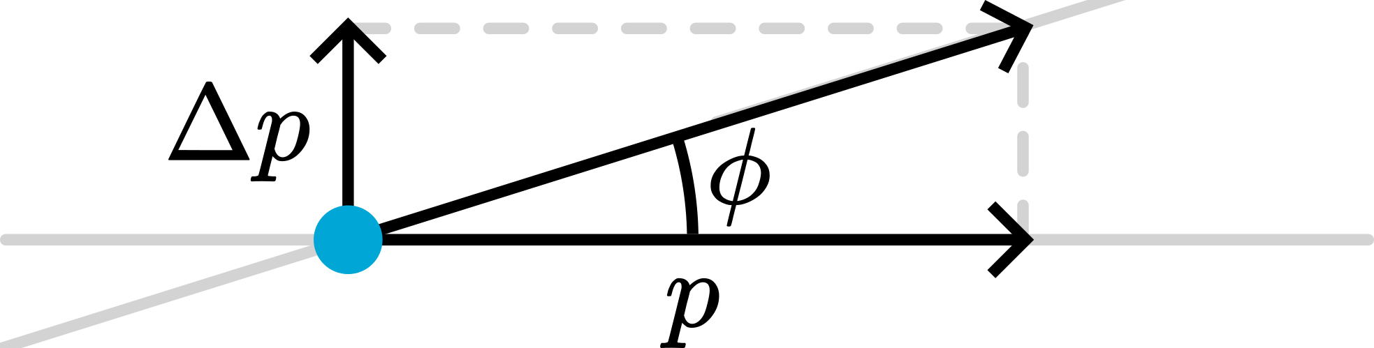
Figure 8:Relation of angle of deflection and change in momentum.
The momentum change is due to the force working for a time period on the particle:
The time the particle is in the atom is estimated as follows: the particle has a velocity and it has to travel a distance through the atom, thus . We assume that the change in momentum is small, so that we can still use as an estimate of the velocity with which the -particle travels.
If we put everything together, we find:
We have used the known charge of a gold atom () and that of the -particle, the radius of the gold atom and the incoming velocity of the -particle, .
With this estimate and the fact that Rutherford’s gold foil was about 400 atoms thick, there is no way that we can explain -particles bouncing back.
Rutherford and his colleagues, had no other option than to conclude that the positive charge of the gold atom must be confined to a much smaller part of space. After all, the only parameter in our estimate that is not measured is . That was estimated based on the plum pudding model.
They redid the calculation, but now with as a free parameter to be backed out of the calculation. They changed the requirement of small scattering angles (i.e. small deviation from the original path) to the experimental finding that scattering angles of about 180° were possible. That gave that is on the order of .
Conclusion: the atom has a nucleus, which contains all of its positive charge and is much smaller than the atom itself. The electrons must orbit this nucleus as a mini-solar system. These electrons ‘define’ the size of the atom.

Figure 9:Rutherford’s model of an atom.
This new model would spark a whole new set of questions, setting up one of the biggest changes in physics: Quantum Theory.
Collapse of matter?
An immediate consequence of this new view on atoms and matter came from the analogy with Newton’s work on the solar system and the Kepler Laws. In the case of the sun and planets, the interaction force is gravity: . When dealing with a nucleus with its orbiting electrons the interaction force is the Coulomb force: .
As both Gravity and Coulombs forces are central, conservative forces and are inversely proportional to the square of distance between the two interacting particles, the motion of a ‘tiny’ planet around the ‘massive’ sun is mathematically completely analogous to that of a ‘tiny’ electron around its ‘massive’ nucleus.
Thus an electron orbits the nucleus in an ellipse. Consequently, it is in a permanent state of acceleration. However, from Maxwell’s theory of electromagnetism it is well known (already in the times of Rutherford as the theory of Maxwell dates back to around 1860) that accelerating charged particles radiate energy in the form of electromagnetic waves. This means that the electron constantly looses energy and thus moves to an elliptical orbit closer to the nucleus until, eventually, its orbit collapses onto the nucleus. This process would go very fast and matter in its present form could not exist. Now we know that the idea of an atom being a miniature solar system is wrong. But questions and dilemmas like these grew very quickly, giving rise to quantum mechanics and opening a whole new world: a completely different picture of things at small scales. A world with new rules and new consequences, where our intuition, based on daily life and large-scale structures composed of many, many atoms, fails.
Scattering Theory
The work of Rutherford and co-workers forms the start of a new branch of physics: nuclear physics. By using radiation in the form of X-rays (i.e. high energy photons) and electrons or protons, physicists are able to probe the internal properties of molecules, atom, nuclei and even elementary particles (or at least, what we once thought were elementary particles).
The idea is to send high energy particles towards the object of investigation and look at the scattering that is a consequence of the interaction between the object and the incoming particles. The internal structure of the object dictates the scattering. Thus, by measuring the scattering features and back tracing the underlying physical interaction can be found.
It is done with facilities of a very large scale to research particles at the smallest scales. For instance, in CERN researchers accelerate particles (protons, electrons, etc) to velocities almost the speed of light. Then, they let these particles collide, that is undergo interactions involving enormous amounts of energy, and measure the fragments and all kind of exotic particles that result from these collisions.
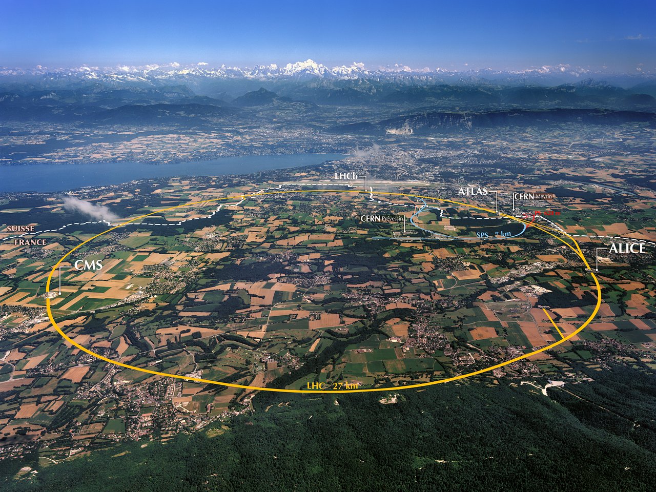
Figure 10:Circular Accelerator of CERN depicted in its environment. ESO/José Francisco, licensed under CC-BY 4.0.
The principles used in scattering can be illustrated by revisiting Rutherford’s experiment.
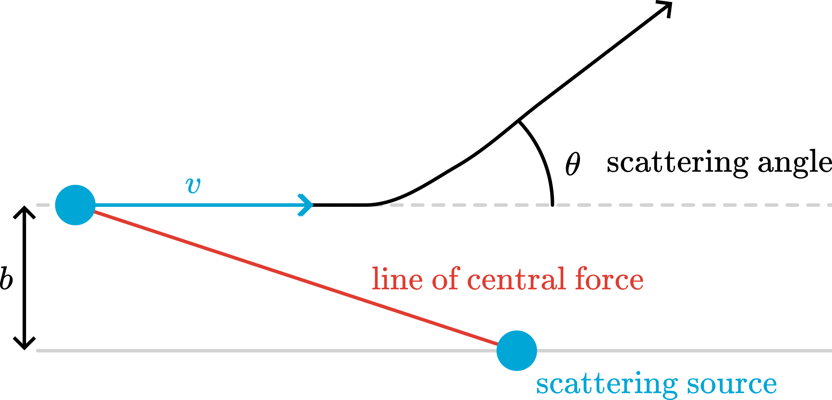
Figure 11:Scattering of an incoming particle at a fixed source.
Consider Figure 11: a particle of mass and velocity is moving towards a fixed second particle. The latter is fixed in the origin and act like a force-source. The force is central, i.e. works along the direction of the red line in Figure 11. In the drawing the forces is repelling and the incoming particle will deviate from its straight line. Eventually it will continue moving over a straight line, when the influence of the force is no longer felt. The angle of the new direction with the incoming one, is , the scattering angle. We are looking for the relation between , the distance at which the incoming particle would have passed by the origin if there was no force and the scattering angle .
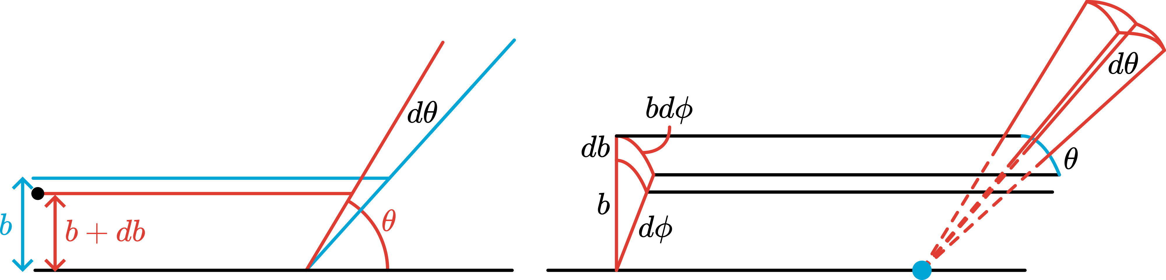
Figure 12:left: scattering in 2D, right: scattering in 3D.
In Figure 12 scattering in a 2D world and in the 3D world is schematically depicted. In the 3-dimensional world the scattering takes place in the solid angle . Like the 2D equivalent, where the scattering angle can go from 0 to (that is the full circle), in 3D it goes from 0 to reflecting that it is now a full sphere.
Kinetic theory of gases
Already in the 18 century, work was done on what we call the kinetic theory of gases. The Swiss scientist Daniel Bernoulli proposed that gases were a large collection of molecules, i.e tiny particles moving in all directions. According to Bernoulli, their collision with walls was felt macroscopically as pressure and their averaged kinetic energy was in essence the temperature of the gas.
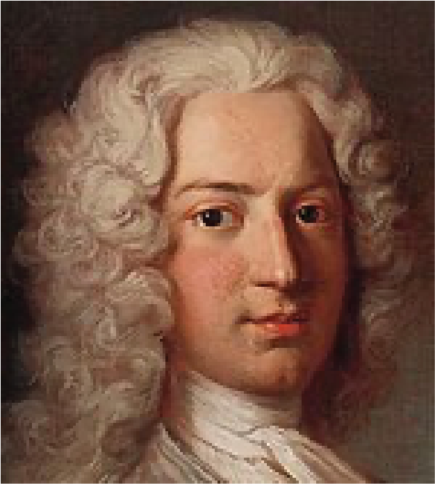
(a)Daniel Bernoulli (1700-1782). From Wikimedia Commons, licensed under CC-BY-SA 4.0.
(b)James Clerk Maxwell (1831-1879) From Wikimedia Commons, public domain
Figure 13:Two famous scientists working on the physics of gases.
It took a while before these ideas were accepted, partly because the law on conservation of energy was not fully developed. Moreover, people had difficulty accepting that at a molecular level collisions could be perfectly elastic.
With the further development of Thermodynamics, the kinetic theory of gases also refined. In 1856, August Krönig came up with a simple kinetic model for gases in which he only considered the possibility of translational motion of the molecules. In essence, he treated gas molecules as point particles. A year later, Rudolf Clausius incorporated the possibility of rotation and vibrations. Two years after this, James Clerk Maxwell continued along this line. He found the velocity distribution of the molecules and established a firm connection between temperature and the average kinetic energy of a molecule. However, he also noted that the theoretical predictions were not in line with experiments. What was the problem?
Specific heat of gases
For ideal gases, we have the ideal gas law: with the number of moles of the gas in question. Or written in terms of number of molecules, , it reads as: , being the Boltzmann constant.
The ideal gas law helps in understanding how gases behave under changing conditions. For instance, if we compress a given amount of gas, we may expect that the pressure goes up. But we also see that this depends on whether or not the temperature changes. And in principle the temperature will change.
If we would do a compression experiment with a fixed number of molecules, , and we would compress the gas such that no heat can escape from the container, then the changes in temperature, volume and pressure are such that . This is called adiabatic compression. The quantity is the ratio of the specific heat at constant pressure over the specific heat at constant volume. Both these quantities are easily measured in experiments and, hence, can be found for many gases.
The kinetic theory predicts for various classes of gases. For instance, for monatomic gasses as Helium, it is ; for diatomic gases, such as Oxygen or Hydrogen, it should be . And so on. Moreover, does, according to the kinetic theory, not depend on temperature.
In the table below, the ratio of the specific heats is listed for a number of gasses.
| Gas | kin. gas. th. | |
|---|---|---|
| He | 1.663 | 1.667 |
| Ne | 1.667 | 1.667 |
| Kr | 1.656 | 1.667 |
| Br | 1.28 | 1.286 |
| Cl | 1.34 | 1.286 |
| H | 1.405 | 1.286 |
| N | 1.40 | 1.286 |
| O | 1.395 | 1.286 |
As we see, for the noble gases it is quite ok (at !), but not so for the diatomic gases.
For really high temperatures () for both O and H, it is close to 1.286. But if we go to low temperature, their respective ’s increase and reaches a value of 1.66 for H! Hence, Maxwell concluded that the laws of classical mechanics could not be the final answer.
The problem with Maxwell’s equations
In the early 1860s Maxwell extended Ampères’ law, in combination with Gauss and Faraday laws. This led to four coupled differential equations describing the generation of electromagnetic fields from charges and currents. They are now just known as the Maxwell equations. They read in modern (differential) notation as follows for the electric and magnetic field in free space
With the charge density distribution and the electric current density, and constants the vacuum permittivity and the vacuum magnetic permeability.
You will learn all about Maxwell’s equations in classes on electromagnetism. The mathematics of these equations is quite difficult as each equation is and the equations are coupled.
In vacuum ( and ) we can simplify these equation. Furthermore, we could look at 1-dimensional cases, that is the electric field has only a component which is only depending on time and the -coordinate. This leads us to the wave equation
This equation describes the propagation of the electric field through vacuum (you can of course derive the same equation for the magnetic field). In the wave equation a second derivative in space is coupled to a second derivative in time. The solution to this differential equation is , with the wave number related to the wave length and the angular frequency to the frequency according to (see also Oscillations). Like for all waves, the frequency, wave length and velocity of the wave are coupled: with the speed of the wave, i.e. in this case the speed of light.
Light is identified as an electromagnetic wave and from the wave equation we see that the wave velocity is given by
If the Maxwell equations are laws of physics all inertial observers must be able to write down the equation in the same form. Therefore for an observer , traveling at constant velocity with respect to , we would write down the wave equation for a field that propagates only along the -direction with amplitude in the -direction (without loss of generality) as
This has exactly the same form as for which is needed if it should represent a physical law. However, for the speed of the wave is also given by . As the speed is covered by universal constants , the speed is the same of and or in other words ! This is not what should happen! From the Galilean Transformation we know that we should find the same form, but with , with the relative velocity of the two observers.
If we apply the coordinate transformation from according to the Galilean Transformation, the wave equation reads as
Now we still need to find a transformation (and trying to retrieve the general form of the wave equation. But there is no such transformation! Therefore, the wave equation of electromagnetic waves is not Galilei invariant at all! This was a serious issue at the time.
Hypothesis of the aether
As light is a wave, people naturally thought there must be a medium to transport the wave, something must be oscillating. Vacuum was considered nothing, not something. A water wave, needs water as medium to transport the wave; the water oscillates. Or take sound waves, they need gas, liquid or a solid to oscillate. What could be the medium that light, electromagnetic waves, use to oscillate? This medium must be all around us, in the space between the sun and earth, just everywhere. To save the Galilei invariance of Maxwell’s equations this also needs to be a very special kind of medium that behaves differently than other media. This strange hypothetical medium was termed aether (ether). The search for the properties of the aether lead to the Michelson-Morley experiment - which showed that there was no aether at all! Lorentz and Fitzgerald found an ad hoc way to save the day by postulating an adapted version of the Galilean Transformation and a contraction of length. Later more about that, and how Einstein showed that all of this ad hoc business is not needed, things follow directly from his second axiom.
The Michelson-Morley experiment
The Michelson-Morley experiment was performed in between 1880-1890 to investigate properties of the hypothetical aether. The experiment returned a null-result, i.e. there was no sign of the existence of the aether - and to this day there is none.
The idea was to check the speed of light for two observers and . One is moving with respect to the other with the highest possible speed, the orbit speed of the earth around the sun . Of course, that is still only 10-4 compared to of the speed of light but the effects could be measured spectroscopically by interference of light.
The experiment essentially consists of a Michelson interferometer. Light is send to a 50/50 beam splitter such that half of the light is reflected towards arm and half is transmitted to arm . The mirrors at the end of each arm reflect the light back. On the way back again, half of the light is transmitted and reflected at the beamsplitter, such that half of the light from both arms is now traveling downwards towards the image plane/camera. At the image plane the light from both arms forms an interference pattern, depending on the path length difference induced by the difference of .
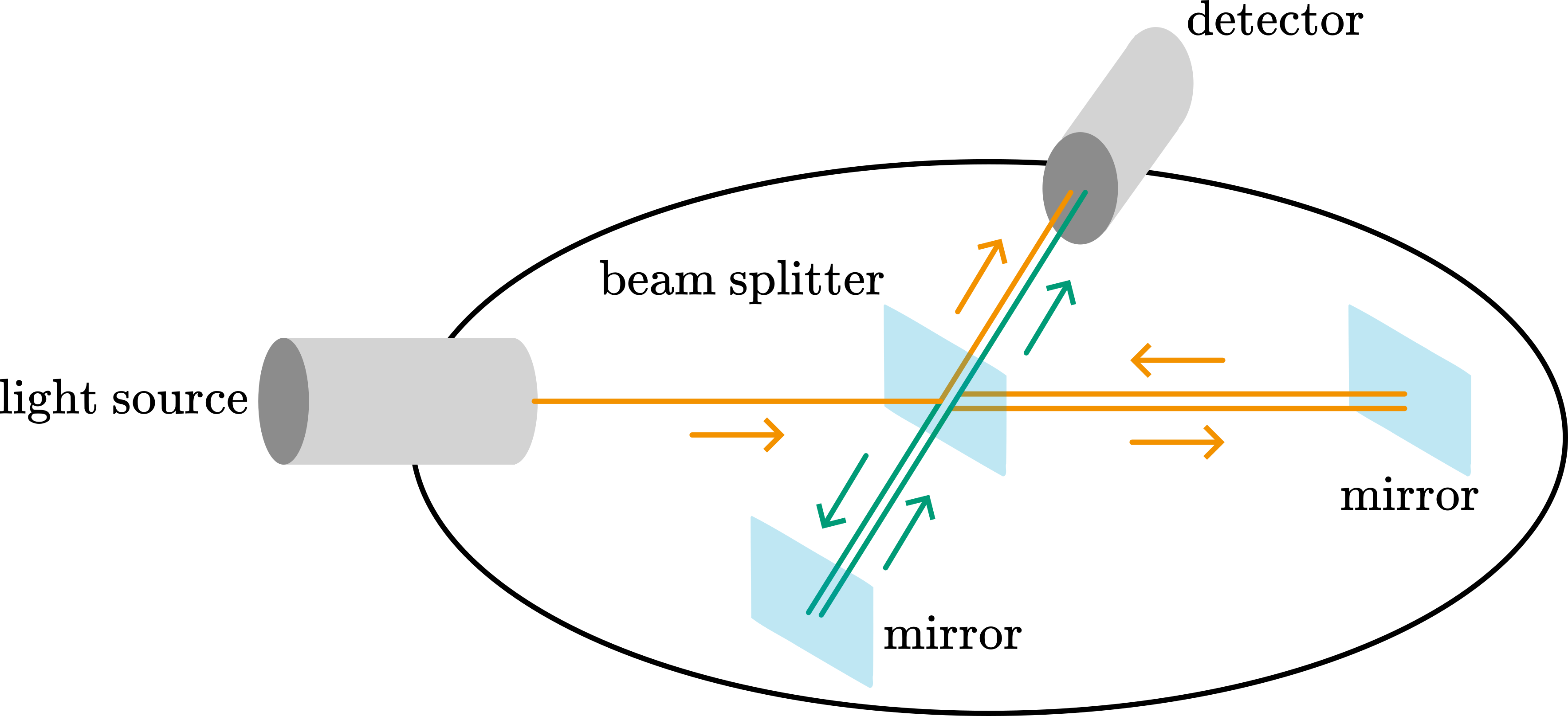
Figure 15:Michelson & Morley setup
The whole setup is mounted for stability on a heavy table that is floating in liquid mercury, to reduce vibrations coupling to the setup. If now one arm is parallel to the earth’s orbit with , while the other is perpendicular to it, there will be some difference between the length of the two paths traveled: . If we rotate the setup by (easily done in the mercury bath), then the roles of and are exchanged, leading to another phase shift . Therefore after rotation the fringes of the interference pattern on the detector should shift as
If we fill in the numbers , and this results in an expected . However, Michelson and Morley found only . The experiment to find the aether failed.[1]
Although the proposed hypothetical medium aether does not exist, as proven a long time ago, the terminology did not drop from everyday language.
Einstein’s axioms
In 1905 Einstein formulated his special theory of relativity with the article Zur Elektrodynamik bewegter Körper, Annalen der Physik, 17:891-921, 1905. He choose the Maxwell equations and the Michelson Morley experiment as a starting point for this argument to arrive at
The laws of physics are the same in all inertial frames of reference.
The velocity of light in vacuum is the same in all inertial frames.
That does not sound like a lot, or world changing, but it certainly was. You can directly see that the second axioms violates Galilean addition of velocities, but that is what was found experimentally by Michelson and Morley!
If you think these two axioms stubbornly through and take their consequences seriously, things get confusing, surprising and almost impossible to believe. Nevertheless, we will do this. Why? Because nature is this way, whether we like it or not.
Back in the days, white light was used for the actual measurement and monochromatic coherent light of e.g. a sodium lamp for alignment. As white light produces a colored interference pattern which is much easier to observe visually. Otherwise temperature changes or vibrations, resulted in constant fringe drift. Today monochromatic laser light can be used in combination with environmental temperature control better than to and sensitive CCD cameras. Today experiments have confirmed the null-result of Michelson and Morley but to much better precision. The anisotropy in the speed of light is .