7.1What are collisions?
In daily life we do understand what a collision is: the bumping of two objects into each other. From a physics point of view, we see it slightly different. The objects don’t have to touch. It is sufficient if they undergo a mutual interaction ‘with a beginning and an end’. What do we mean by this?

Figure 1:Collision of two particles.
Firstly, the mutual interaction means that the objects interact with each other through a mutual force, i.e. a force (pair) that obeys Newton’s third law.
Secondly, we assume that this force works over a small distance only. Or re-phrased we will only consider the situation before the objects feel the force and compare that to after they have felt it. We don’t bother about the details of the motion of the objects during their interaction. Hence, when we depict a collision as in Figure 1, we usually draw the situation before the collision, then some kind of ‘comic way’ of showing the collision and finally we draw the outcome of the collision, so after the interaction. In many cases, people leave the middle part out of their drawing.
There are two principle types of collisions to distinguish: elastic and inelastic collisions. For an elastic collision the kinetic energy is conserved, whereas for an inelastic that is not the case. In the latter case, energy can be converted into deformation or heat.
Since the objects interact under the influence of their mutual interaction, we have conservation of momentum:
Why? No external forces implies constant total momentum.
7.2Elastic Collisions
For an elastic collision the kinetic energy is conserved by definition (next to the conservation of momentum). That is the sum of the kinetic energy before the collision is the same as the sum after the collision. This type of collision is also called hard-ball collision: as with colliding billiard balls no energy is dissipated into heat or deformation.
Figure 3:A simulation on collisions. Try to change the mass, velocity, angle of contact...
For elastic collisions the interaction force needs to be conservative. Then, a potential energy exists. And this energy is such that the objects have the same potential energy before as after the collision. Consequently energy conservation leads to:
7.2.1Solving collision problems
Given a collision experiment where the initial situation before the collision is known, how do we compute the situation after the collision? What will the velocities of the object be?
Consider a head-on collision of two point particles on a line as shown in Figure 4. One particle with mass is initially at rest (), the other with mass has velocity . What are the velocities of the particles after the collision?

Figure 4:Example of a 1D elastic collision.
We can write down two equations using conservation of momentum and kinetic energy before and after the collision
We have two equations and two unknowns , therefore we can in principle solve this problem. The question is, what is the best strategy to do so? A strategy is needed especially since one equation involves the square of the velocity.
We first bring the velocities and to the same side.
Now we divide the two equations (verify yourselves!), this makes the solution very easy as the squares of the velocities always divide out.
We can use this to find both unknowns by smartly adding equations and . Smartly in the sense that we can multiply either of the equations with a scalar in such way that one quantity can be discarded.
This solution strategy always works. NB: you need to practice this. Although it is conceptually easy, we often see that students have problems when actually solving for the 2 unknowns.
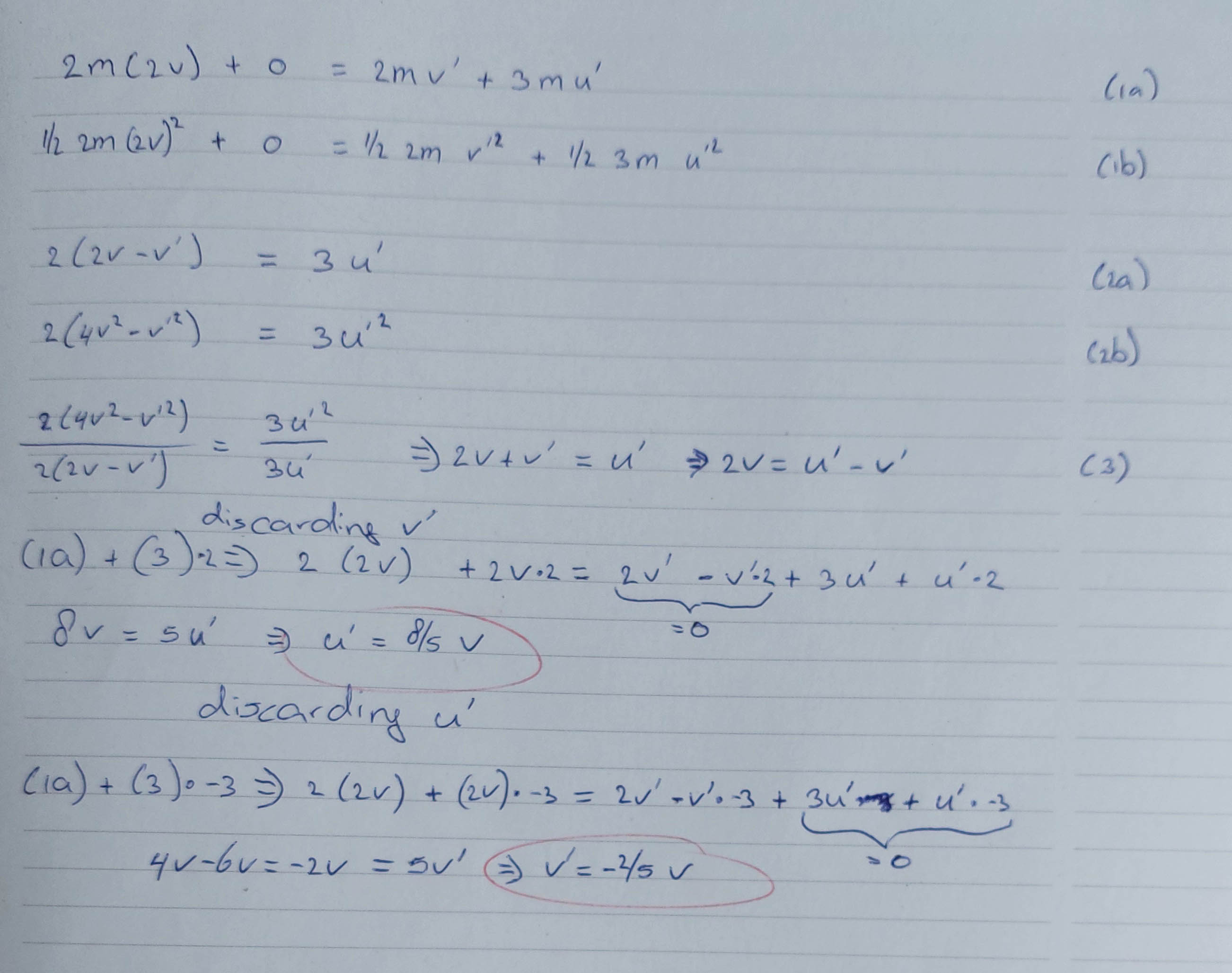
Figure 5:Solving the problem
Actually, now we think about this strategy: isn’t it strange, the kinetic energy equation is squared in our unknowns. Shouldn’t we expect 2 solutions?
The answer is yes: there ought to be 2 solutions. Where is the second one? Note that when dividing the two equations, we have to make sure that we do not divide by 0. It is very well possible that we do so: suppose , then also and we can not do the division. But what does that mean: and ? Well, of course, then we have after the collision that the incoming particle still has velocity and the other particle is still at rest.
In retrospect: of course this must be one of the solutions to the problem. We haven’t specified anything about the interaction force. But suppose it is absent, that is, the particles don’t interact at all. Then of course the situation before the collision (a bit strange calling this a collision, but anyway), will still be present after the ‘collision’. If nothing happens to the particles, then obviously the sum of the momentum as well as of the kinetic energy stays the same. This actually provides a great check of your work: do you recover the initial conditions?
7.2.2Collisions in a plane
Consider now a 2D elastic collision such that the two particles collide in the origin, Figure 6.

Figure 6:Example of a 2D elastic collision.
If we write down the equation of conservation of momentum (in components) and of kinetic energy, we get
Now we have 4 unknowns () but only 3 equations. The outcome seems not to be determined by the initial condition... Of course, that cannot be the case (Think shortly why?). The outcome is fully determined by the initial conditions, but we did not set up the equations in the best way because we did not first transform the problem into a 1D problem such that the collision is head-on.
We can use a Galilean Transformation to put one particle at rest. Here we set the blue particle to rest by subtracting from its velocity, that is we move with the blue particle (prior to the collision). The corresponding Galilean Transformation is
The red particle now has velocity . The problem is still 2D.

Figure 7:Applying the Galilean Transformation.
Next, we can rotate the coordinate system, to obtain a 1D head-on collision that we can solve as above.

Figure 8:Rotating the coordinate system.
We see that we now have a 1-dimensional elastically collision with a particle of mass coming in over the -axis with velocity . It will collide with a particle of mass which is at rest. We know how to solve this problem and find the velocities of both particles after the collision. If we do this, we find that after the collision the velocity of the blue particle is and of the red particle . Note that we have specified these velocity in the coordinate system.
Next steps would be to convert the velocities back to the initial coordinate frame. That is a bit cumbersome, but again conceptually easy. The final answer in the original frame of reference is:
The 3Blue1Brown series on linear algebra describes the linear transformations above in a mathematical way. Using linear algebra, above computations will become easier.
Source
import numpy as np
import matplotlib.pyplot as plt
import matplotlib.animation as animation
from IPython.display import display, HTML, Math
import ipywidgets as widgets

# Constants
m1_init = 1
m2_init = 1
v1x_init = 1
v1y_init = 0
v2x_init = 0
v2y_init = 1

x1_init = -1
y1_init = 0
x2_init = 0
y2_init = -1


# Time setup
dt = 0.05
time_max = 1
times_neg = np.arange(-time_max, dt, dt)
times_pos = np.arange(dt, time_max, dt)
times = np.arange(-time_max, time_max, dt)
Ntimes = len(times_neg) + len(times_pos)

# Widget slider mass 1
mass1_slider = widgets.FloatSlider(
    value=1,
    min=1,
    max=5,
    step=1,
    description='m1:',
    continuous_update=False
)

# Widget slider mass 2
mass2_slider = widgets.FloatSlider(
    value=1,
    min=1,
    max=5,
    step=1,
    description='m2:',
    continuous_update=False
)

# Widget slider velo v1x
velocity1x_slider = widgets.FloatSlider(
    value=1,
    min=1,
    max=5,
    step=1,
    description='v1x:',
    continuous_update=False
)

# Widget slider velo
velocity1y_slider = widgets.FloatSlider(
    value=0,
    min=-3,
    max=3,
    step=1,
    description='v1y:',
    continuous_update=False
)

# Widget slider velo v2x
velocity2x_slider = widgets.FloatSlider(
    value=0,
    min=-3,
    max=1,
    step=1,
    description='v2x:',
    continuous_update=False
)

# Widget slider velo
velocity2y_slider = widgets.FloatSlider(
    value=1,
    min=1,
    max=3,
    step=1,
    description='v2y:',
    continuous_update=False
)

def CalcCol(m1_init,m2_init,v1x_init,v1y_init,v2x_init,v2y_init):
    #initiallise m's and v's
    v1x, v1y = v1x_init, v1y_init
    v2x, v2y = v2x_init, v2y_init
    m1, m2 = m1_init, m2_init
    cos_2 = v2x/np.sqrt(v2x*v2x+v2y*v2y)
    sin_2 = v2y/np.sqrt(v2x*v2x+v2y*v2y)

    # new velocities after collision
    # velo center of gravity
    Vcg_x=(m1*v1x+m2*v2x)/(m1+m2);
    Vcg_y=(m1*v1y+m2*v2y)/(m1+m2);
    #relative velos before coll in COG
    u1x=v1x-Vcg_x;
    u1y=v1y-Vcg_y;
    u2x=v2x-Vcg_x;
    u2y=v2y-Vcg_y;
    u1=np.sqrt(u1x*u1x+u1y*u1y);
    u2=np.sqrt(u2x*u2x+u2y*u2y);
    cos_1=u1x/u1;
    sin_1=u1y/u1;
    cos_2=u2x/u2;
    sin_2=u2y/u2;

	#rotation matrix to rotatate to 1D picture -> particles moving over x-axis
    A11=cos_1;
    A12=sin_1;
    A21=-sin_1;
    A22=cos_1;
    uac1x=A11*u1x+A12*u1y;
    uac1y=A21*u1x+A22*u1y;
    uac2x=A11*u2x+A12*u2y;
    uac2y=A21*u2x+A22*u2y;

    #new velos: do a 1D collision
    wac2x=((1-m1/m2)*uac2x+2*m1/m2*uac1x)/(1+m1/m2);
    wac1x=uac2x-uac1x+wac2x;
    wac1y=0;
    wac2y=0;
    #rotate back
    w1x=A11*wac1x-A12*wac1y;
    w1y=-A21*wac1x+A22*wac1y;
    w2x=A11*wac2x-A12*wac2y;
    w2y=-A21*wac2x+A22*wac2y;
    #transform back to lab frame
    vnew1_x=w1x+Vcg_x;
    vnew1_y=w1y+Vcg_y;
    vnew2_x=w2x+Vcg_x;
    vnew2_y=w2y+Vcg_y;
    if vnew1_x <0.0001:
        alpha_1 = 90
    else:
        alpha_1 = round(np.arctan(vnew1_y / vnew1_x)/np.pi*180/10)*10;
    if vnew2_x <0.0001:
        alpha_2 = 90
    else:
        alpha_2 = round(np.arctan(vnew2_y / vnew2_x)/np.pi*180/10)*10;

    return vnew1_x, vnew1_y, vnew2_x, vnew2_y, alpha_1, alpha_2

def generate_animation(m1_init,m2_init,v1x_init,v1y_init,v2x_init,v2y_init):
    v1x, v1y = v1x_init, v1y_init
    v2x, v2y = v2x_init, v2y_init
    x1 = v1x*(-time_max)
    x2 = v2x*(-time_max)
    y1 = v1y*(-time_max)
    y2 = v2y*(-time_max)

    m1, m2 = m1_init, m2_init

    u1_x, u1_y, u2_x, u2_y, a1, a2 = CalcCol(m1_init,m2_init,v1x_init,v1y_init,v2x_init,v2y_init)

    # Position history
    x1_list, y1_list = [], []
    x2_list, y2_list = [], []

    for t in times_neg:
        x1_t = v1x * t
        y1_t = v1y * t
        x1_list.append(x1_t)
        y1_list.append(y1_t)
        x2_t = v2x * t
        y2_t = v2y * t
        x2_list.append(x2_t)
        y2_list.append(y2_t)

    for t in times_pos:
        x1_t = u1_x * t
        y1_t = u1_y * t
        x1_list.append(x1_t)
        y1_list.append(y1_t)
        x2_t = u2_x * t
        y2_t = u2_y * t
        x2_list.append(x2_t)
        y2_list.append(y2_t)

    # Create figure and axes
    fig, ax = plt.subplots(figsize=(6, 6))
    ax.set_xlim(-6, 6)
    ax.set_ylim(-6, 6)
#    ax.set_yticks([])
    ax.set_title("2D Elastic Collision")
    ax.plot([-6,6],[0,0], color='grey')
    ax.plot([0,0],[-6,6], color='grey')

    p1, = ax.plot([], [], 'ro', markersize=6, label='Particle 1')
    p2, = ax.plot([], [], 'bo', markersize=6, label='Particle 2')
    p1_line_f, = ax.plot((x1_list[0],x1_list[0]),(y1_list[0],y1_list[0]),'r-')
    p1_line_a, = ax.plot((0,0),(0,0),'r-')
    p2_line_f, = ax.plot((x2_list[0],x2_list[0]),(y2_list[0],y2_list[0]),'b-')
    p2_line_a, = ax.plot((0,0),(0,0),'b-')
    ax.grid()
    ax.legend(loc='upper right')

    def init():
        p1.set_data([], [])
        p2.set_data([], [])
        return p1, p2

    def update(i):
        p1.set_data([x1_list[i]], [y1_list[i]])
        p2.set_data([x2_list[i]], [y2_list[i]])
        if i < len(times_neg):
            p1_line_f.set_data((x1_list[0],x1_list[i]),(y1_list[0],y1_list[i]))
            p2_line_f.set_data((x2_list[0],x2_list[i]),(y2_list[0],y2_list[i]))
        else:
            p1_line_a.set_data((0,x1_list[i]),(0,y1_list[i]))
            p2_line_a.set_data((0,x2_list[i]),(0,y2_list[i]))
        return p1, p2


    ani = animation.FuncAnimation(fig, update, frames=Ntimes, init_func=init,
                                  interval=50, blit=True)

    plt.close(fig)
    return HTML(ani.to_jshtml())

# Show slider and link it to animation
widgets.interact(generate_animation,
    m1_init = mass1_slider, m2_init = mass2_slider,
    v1x_init = velocity1x_slider, v1y_init = velocity1y_slider,
    v2x_init = velocity2x_slider, v2y_init = velocity2y_slider
    );
7.3Collisions in the Center of Mass frame
There is a special frame of reference: the Center of Mass (CM) frame. Its origin is defined with respect to the lab frame as
We will introduce this formally in the next chapter.
As the mass is conserved during a collision we have
- and
- as the momentum is conserved ,
we see that the velocity of the CM does not change before and after collision
Instead of working in the lab frame we can use the CM frame. A sketch of the coordinates and vectors is given in the figure below.

Figure 10:Center of mass.
For the relative coordinates it holds that . Considering two particles: The relative distance is Galilei invariant.
Using this property we express the vectors and in terms of the relative distance vector for and with the so-called reduced mass (see next chapter). Therefore
This means the momenta of both particles are always equal in magnitude and opposed in direction in the CM frame. Only the orientation of the pair can change from before to after the collision.

Figure 11:Collision in center of mass frame.
7.4Computational
For collisions with only a ‘few’ particles, it is doable to calculate the outcomes by hand. That is, if there are no angles involved. It becomes more difficult if we want, for instance, compute a box with 104 particles. Such a simulation may provide key insights in thermodynamic behavior.
Computing multiple collisions by hand is quite challenging, but can be done ‘easily’ with the computer. Figure made by A. Greg, public domain
In computing collissions, we can make use of the general solution:
as derived in Craver (2013).
Figure made by Simon Steinmann, CC-SA
In an angle-free representation - using vectors rather than angles, the changed velocities are computed using the centers and at the time of contact as:
In Python this would become:
vA_new = vA - 2 * mB / (mA + mB) * np.dot(vA - vB, rA - rB) / (1e-12+np.linalg.norm(rA - rB))**2 * (rA - rB)
vB_new = vB - 2 * mA / (mA + mB) * np.dot(vB - vA, rB - rA) / (1e-12+np.linalg.norm(rB - rA))**2 * (rB - rA)
Note that a vary small number is added () to prevent that the denominator does not become 0.
7.5Inelastic Collisions
For inelastic collisions only the momentum is conserved, but not the kinetic energy. The kinetic energy after the collision is always less than before the collision. As the total energy is conserved, some kinetic energy is converted to deformation or heat.
The amount of “inelasticity” or loss of energy can be quantified by the coefficient of restitution
For the collision is fully inelastic, for it is fully elastic.
- Craver, W. (2013). Elastic Collisions. https://williamecraver.wixsite.com/elastic-equations