4.1Torque & Angular Momentum
From experience we know that if we want to unscrew a bottle, lift a heavy object on one side, try to unscrew a screw, we better use ‘leverage’.

Figure 1:Lifting is easier using leverage.
With a relatively small force , we can lift the side of a heavy object. The key concept to use here is torque, which in words is loosely formulated: apply the force using a long arm and the force seems to be magnified. The torque is then force multiplied by arm:
This is, of course, too sloppy for physicists. We need strict, formal definitions. So, we put the above into a mathematical definition.
That is: torque (or krachtmoment in Dutch) is the cross product of ‘arm’ as a vector(!) and the force. We notice a few peculiarities.
- like force, torque is a vector. That is: it has a magnitude and a direction. In principle: three components.
- its direction is perpendicular to the force vector and perpendicular to the arm .
- the arm is not a number: it is a vector!
We further know from experience that we can balance torques, like we can balance forces. Rephrased: the net effect of more than one force is found by adding all the forces (as vectors!) and using the net force in Newtons Second Law: . From Newtons First Law, we immediately infer: if then the object moves at constant velocity. We can move with the object at this speed and conclude that it from this perspective has zero velocity: it doesn’t move, i.e. it is in equilibrium.
The same holds for torque: we can work with the sum of all torques that act on an object: . And if this sum is zero, the object is in equilibrium.
However, there is a catch: using torques requires that we are much more explicit and precise about the choice of our origin. Why? The reason is in the ‘arm’. That is only defined if we provide an origin.
4.1.1The seesaw and torque
Let’s consider a simple example (simple in the sense that we are all familiar with it): the seesaw.

Figure 2:An adult (left) and a child (right) on a seesaw.
It is obvious that the adult -seesawing with the child- should sit much closer to the pivot point than the child. That is: we assume that the mass of the adult is greater than that of the child.
Let’s turn this picture into one that captures the essence and includes the necessary physical quantities, and then draw a free-body diagram.

Figure 3:Free-body diagram of the seesaw and the masses.
What did we draw?
- The force of gravity acting on the two masses and . That is obvious: without forces nothing will happen and there is nothing to be analyzed.
- The ‘reaction forces’ from the seesaw on both masses. Why? If the seesaw is in equilibrium, then each of the masses is in equilibrium and the sum of forces on each mass must be zero.
- The distance of each of the masses to the pivot point. Why? Leverage! The heavy must be closer to the pivot point the get equilibrium.
- An origin . Why? We need a point to measure the ‘arm’, ‘leverage’, from.
- The -coordinate. Why? We deal with forces in the vertical direction. Hence a coordinate, a direction that we all use, is handy.
Analysis
Time for a first analysis: what keeps this seesaw in equilibrium?
- The sum of forces on each of the masses is zero. As gravity pulls them down, the seesaw must exert a force of the same magnitude but in the opposite direction. These are the green forces.
- With this idea we have the masses in equilibrium, but not necessarily the seesaw. Why? We did not consider forces on the seesaw. Which are these: (a) the reaction force (i.e. the N3 pair) of the green force from the seesaw on mass . We did not draw that! Similarly, for the mass .
- Now that we focus on the seesaw itself: this is in equilibrium (that is given), but there are two forces acting on it in the negative -direction as we found in (2). Even if we consider the mass of the seesaw: that will not help, gravity will pull it downwards. What did we forget? The force at the pivot point, of course! The pivot will exert an upward force, preventing the seesaw from falling down. For simplicity, we assume that the seesaw has zero mass. Thus, there are three forces acting on it: , , with .
Let’s redraw, now concentrating on the forces on the seesaw.

Figure 4:Free-body diagram of the seesaw.
Analysis part 2
We know that the seesaw is in equilibrium, thus
This guarantees that the seesaw does not change its velocity, and as it does not move at some time , it doesn’t move for all .
But this doesn’t guarantee that the seesaw doesn’t rotate around the pivot point. For that we need that the ‘leverages’ on the left and right side ‘perform’ the same.
Making this precise: the torques exerted on the seesaw must also equate to zero.
We have 3 forces, thus 3 torques: with arm , with arm and with arm zero.
Now we need to be even more precise: torque is a vector and it is made as a cross product of the vector ‘arm’ and the force.
We have already drawn an -coordinate in the figure, that will allow us to write the ‘arm’ as a vector. After all, we need to evaluate the cross product . We do that for the three forces, starting on the left:
We have used here, that the cross product of with is equal to with the unit vector in the -direction pointing into the screen.
Similarly for the force coming from the small mass on the right side:
Finally, the torque from the force exerted by the pivot point:
Next, we evaluate the total torque:
In order for the seesaw not to start rotating, we must have that the torque is zero and thus:
A result we expected: the greater mass should be closer to the pivot point.
4.1.2Different origin
So far, so good. But what if we had chosen the origin not at the pivot point, but somewhere to the left? Then all ‘arm’ will change length. And all torques will be different. Wouldn’t that make ?
No, it wouldn’t! Let’s just do it and recalculate. In the figure below, we have moved the origin to the left end of the seesaw. The distance from the heavy mass to the origin is (green arrow).

Figure 5:Free-body diagram with the origin located at the seesaw’s end.
We still have that the sum of forces is zero. But what about the sum of torques? Obviously, the choice of the origin can not affect the seesaw: it is still in balance, regardless of our choice of the origin. Let’s see if that is correct:
We have drawn the three unit vectors in the figure. We will use again: . This simplifies the torque equation above to:
This is clearly more complicated than the expression we had with the first choice of the origin. Moreover, the force from the pivot point shows up in our expression.
Luckily, we have equilibrium. Hence: . We substitute this into our torque equation:
Which is exactly the same expression as we found before. So, indeed, the choice of the origin doesn’t matter.
Conclusion
For equilibrium we need that the sum of torques is zero:
4.2Angular Momentum
From our seesaw example we learn: the seesaw can only be in equilibrium if the sum of torques is zero. What if this sum is non-zero? That is, a net torque operates on the seesaw.
We know that the seesaw will rotate and in order to balance it, we have to shift at least one of the masses.
In which direction will it rotate?
Before answering: first we need to think about direction of rotation. Does it have direction and if so: how do we make clear what that is?
Again the seesaw will give guidance. Suppose we remove the smaller mass all together. Then, it is obvious: the ‘heavy’ left side will rotate to the ground and the light right side upwards. From the point of view we are standing: the seesaw will rotate counter clockwise.
We will use the corkscrew rule or right hand rule to give that a direction: rotate a corkscrew clockwise and the screw will move into the cork away from you; rotate a corkscrew counter clockwise and it will move out of the cork, towards you. Of course, in stead of a corkscrew you can think of a screwdriver or a water tap: closing is rotating 'clock wise, opening the tap is counter clockwise.

Figure 6:The rotation is given by the black arrow. You can find it by using the corkscrew rule: rotating a corkscrew as the blue arrow indicates gives that the screw moves forward like the black arrow.
With this, we can define the direction of rotation better than via clock or counter clock wise. In our seesaw example, we will say: if the seesaw rotates clockwise, its rotation is described by a vector that points in the positive -direction as given in the figure, that is pointing into the paper (or screen).
Now, we can couple this to the direction of the torque. We saw -taking the origin at the pivot point- two torques acting on the seesaw. The large mass has its torque pointing in the negative -direction: it points out of the screen/paper. And this torque tries to rotate the seesaw counter clockwise. On the other hand, the small mass has a torque pointing in the positive -direction which is in line with it trying to rotate the seesaw clockwise.
Which of the two is ‘strongest’ determines the direction of rotation: if then the net torque is in the minus- direction. That is, the torque of the larger mass is more negative than the smaller one is positive: and the net torque points towards us.
The quantity that goes with this, is the angular momentum. It is defined as
Note that it is a cross product as well. Hence it is a vector itself. Further note that . The order matters! First then . If you do it the other way around, you unwillingly have introduced a minus sign that should not be there.
Furthermore, note that since , is perpendicular to the plane formed by and .

Figure 7:Angular momentum of a particle at a certain position with momentum.
4.2.1Torque & Analogy to N2
Angular momentum obeys a variation of Newton’s second law that ties it directly to torque.
Thus, we find a general law for the angular momentum:
Again, note that the right hand side is a cross product, so the order does matter.
With the torque denoted by , we have
then we can write down an equation similar to N2 but now for angular motion
where the force is replaced by the torque and the linear momentum by the angular momentum.
NB: Note that the torque and angular moment change if we choose a different origin as this changes the value of .
It is a common mistake to identify angular momentum with rotational motion. That is not correct. A particle that travels in a straight line will, in general, also have a non-zero angular momentum, see Figure 11. Here we look at a free particle: there are no forces working on it. So it travels in a straight line, with constant momentum.

Figure 11:Angular momentum of a free particle.
However, the particle position does change over time. So: is its angular momentum constant or not?
That is easy to find out. We could take ‘N2’ for angular momentum:
Clearly, the angular momentum of a free particle is constant. Moreover, the momentum of a free particle is also constant. But what about the position vector: isn’t that changing over time and eventually becomes very, very long? Why does that not change ?
Take a look at Figure 12. We have chosen the -plane such that both and are in it. Furthermore, we have taken it such that is parallel to the -axis.

Figure 12:Angular momentum of a free particle is constant.
At some point in time, the particle is at position . Its angular momentum is perpendicular to the -plane and has magnitude . Later in time it is at position . Still, its angular momentum is perpendicular to the -plane and has magnitude , indeed identical to the earlier value. This shows that indeed the angular momentum of a free particle is constant.
4.3Examples & Exercises
Solution to Exercise 1
The particle falls under a force that points in the negative -direction. As a consequence, it will start moving vertically downwards:
Thus, we find for the momentum om the particle: .
The position of follows from:
We can now compute the angular momentum:
Thus, the angular momentum is pointing in the negative -direction and increases linearly with time in magnitude.
We could have tried to find this via the variation of N2 for angular momentum. Now, we need to compute the torque on and solve . This goes as follows:
And thus:
To get any further, we need information about . From the -component of N2 we know (see above): . If we plug this in, we get:
where we have used:
Solution to Exercise 2
We can follow the same procedure as in exercise (6.1). But now, the outcome of the -component of N2 changes.
Thus, we find for the momentum om the particle: .
The position of follows from:
We can now compute the angular momentum:
Thus, the angular momentum still points in the negative -direction but increases quadratically with time in magnitude.

Solution to Exercise 3
We can take the situation of Exercise 1, but shift our origin such that at . Now the particle will fall along the -axis. It has its momentum also in the -direction and consequently and stays zero!
4.4Central Forces
We have looked at a specific class of forces: the conservative ones. Here we will inspect a second class, that is very useful to identify: the central forces.
A force is called a central force if:
In words: a force is central if it points always into the direction of the origin or exactly in the opposite direction. The reason to identify this class is in the consequences it has for the angular momentum.
Suppose, a particle of mass is subject to a central force. Then we can immediately infer that its angular momentum is a constant:
where we have used that and are always parallel so their cross-product is zero.
The above is rather trivial, but has a very important consequence: a particle that moves under the influence of a central force, moves with a constant angular momentum (vector!) and must move in a plane. It can not get out of that plane. Thus its motion is at maximum a 2-dimensional problem. We can always use a coordinate system, such that the motion of the particle is confined to only two of the three coordinates, e.g. we can choose our plane such that the particle moves in it and thus always has .
Why is this so? Why does the fact that the angular momentum vector is a constant immediately imply that the particle motion is in a plane? The argumentation goes as follows.
Imagine a particle that moves under the influence of a central force. At some point in time it will have position and momentum . Neither of them is zero. We will assume that and are not parallel (in general they will not be). Thus they define a plane. Due to the cross-product is perpendicular to this plane.
A little time later, say later, both position and momentum will have changed. Since the force is central, the force is also in the plane defined by the initial position and momentum. Thus the change of momentum is in that plane as well: . The right hand side is completely in our plane. And thus, the new momentum is also in the plane. But that means that the velocity is also in the same plane. An thus the new position must be in the same plane as well. We can repeat this argument for the next time and thus see, that both momentum and position can not get out of the plane. This is, of course, fully in agreement with the fact that for a central force.
4.5Central forces: conservative or not?
We can further restrict our class of central forces:
In the above, , that is: the magnitude of the force only depends on the distance from the origin not on the direction. Rephrased: the force is spherically symmetric. If that is the case, the force is automatically conservative and a potential does exist.
Both the concept of central forces and potential energy play a pivotal role in understanding the motion of celestial bodies, like our earth revolving the sun. The planetary motion is an example of using the concept of central forces. It is, however, also an example in its own right. Using his new theory, Newton was able to prove that the motion of the earth around the sun is an ellipsoidal one. It helped changing the way we viewed the world from geo-centric to helio-centric.
4.5.1Keppler’s Laws
Before we embark at the problem of the earth moving under the influence of the sun’s gravity, we will go back in time a little bit.
Kepler has formulated three laws that describe features of the orbits of the planets around the sun.
- The orbit of a planet is an ellipse with the Sun at one of the two focal points.
- A line segment joining a planet and the Sun sweeps out equal areas during equal intervals of time (Law of Equal Areas).
- The square of a planet’s orbital period is proportional to the cube of the length of the semi-major axis of its orbit.

Figure 19:Kepler’s 2nd Law of Equal Area.
Source
%pip install ipywidgets
import numpy as np
import matplotlib.pyplot as plt
from ipywidgets import interact
import ipywidgets as widgets

mass_sun = 1.989e30  # kg
mass_halley = 2.2e14  # kg

G = 6.67430e-11  # m^3 kg^-1 s^-2

# perihelion halley
AU = 149e9         #m

v_halley = 54.68e3  # m/s
r_halley = 0.586 * AU  # m

# settings
dt = 24 * 3600  # seconds
t = 75 * 365 * 24 * 3600  # seconds
N = int(t / dt)

# Ic.
v_h = np.zeros((N,2))
v_h[0,:] = [0,v_halley]

r_h = np.zeros((N,2))
r_h[0,:] = [r_halley,0]

t_arr = np.linspace(0,t+dt,N)

# RK4 method
def acceleration(r):
    r_norm = np.linalg.norm(r)
    return -G * mass_sun * r / r_norm**3

for i in range(1, N):
    # r and v at time t
    r0 = r_h[i-1, :]
    v0 = v_h[i-1, :]


    # k1
    k1_v = acceleration(r0) * dt
    k1_r = v0 * dt

    # k2
    k2_v = acceleration(r0 + 0.5 * k1_r) * dt
    k2_r = (v0 + 0.5 * k1_v) * dt

    # k3
    k3_v = acceleration(r0 + 0.5 * k2_r) * dt
    k3_r = (v0 + 0.5 * k2_v) * dt

    # k4
    k4_v = acceleration(r0 + k3_r) * dt
    k4_r = (v0 + k3_v) * dt

    # update velocity and position
    v_h[i, :] = v0 + (k1_v + 2 * k2_v + 2 * k3_v + k4_v) / 6
    r_h[i, :] = r0 + (k1_r + 2 * k2_r + 2 * k3_r + k4_r) / 6

# Plotting the trajectory

def sim_kep(t_sim):

    plt.figure(figsize=(10, 6))
    plt.xlabel('X Position (m)')
    plt.ylabel('Y Position (m)')

    plt.plot(r_h[:, 0], r_h[:, 1], label='Halley\'s Trajectory', color='lightgray')


    # plt.plot(r_h[N, 0], r_h[N, 1], 'r.')

    plt.scatter(0, 0, color='yellow', s=100, label='Sun')  # Sun at origin
    plt.gca().set_aspect('equal')
    # plt.title('Earth Trajectory Around the Sun')
    plt.title('Halley\'s Trajectory Around the Sun')

    for i in range(1,t_sim,int(N/15)):
        plt.plot(r_h[:i, 0], r_h[:i, 1], label='Earth Trajectory', color='black')
        plt.plot(r_h[i, 0], r_h[i, 1], 'r.')
        plt.arrow(0,0,r_h[i, 0], r_h[i, 1], color='darkgreen')

    plt.text(0,5e11, str(int(t_sim/(365)))+'years')
    plt.grid()
    #plt.legend()
    plt.show()

interact(sim_kep, t_sim=widgets.IntSlider(min=0, max=N-1, step=int(N/15), value=1))It is important to realize, that Kepler came to his laws by -what we would now call- curve fitting. That is, he was looking for a generic description of the orbits of planets that would match the Brahe data. He abandoned the Copernicus idea of circles with epi-circles with the sun in the center of the orbit. Instead he arrived at ellipses with the sun out of the center, in one of the focal points of the ellipse.
But, there was no scientific theory backing this up. It is purely ‘data-fitting’. Nevertheless, it is a major step forward in the thinking about our universe and solar system. It radically changed from the idea that the universe is ‘eternal’, that is for ever the same and build up of circles and spheres: the mathematical objects with highest symmetry showing how perfect the creation of the universe is.
Kepler had formulated his laws by 1619 AD. It would take another 60 years before Isaac Newton showed that these laws are actually imbedded in his first principle approach: all that is needed is Newton’s second law and his Gravitational Law.
4.6Newton’s theory and Kepler’s Laws
The planets move under the influence of the gravitational force between them and the sun. We start with inspecting and classifying the force of gravity. Newton had formulated the Law of gravity: two objects of mass and , respectively, exert a force on each other that is inversely proportional to the square of the distance between the two masses and is always attractive. In a mathematical equation, we can make this more precise:
In the figure below, the situation is sketched. We have chosen the origin somewhere and denote te position of the sun and the planet by and . Gravity works along the vector . The corresponding unit vector is defined as .

Figure 20:The sun and a planet.
Newton realized that he could make a very good approximation. Given that the mass of the sun is much bigger than that of a planet, the acceleration of the sun due to the gravitational force of the planet on the sun is much less than the acceleration of the planet due to the sun’s gravity. For this, we only need Newton’s 3rd law:
Hence
Newton concluded, that for all practical purposes, he could treat the sun as not moving. Next, he took the origin at the position of the sun. And from here on, we can ignore the sun and pretend that the planet feels a force given by
with the mass of the sun and that of the planet. is now the distance from the planet to the origin and the unit vector pointing from the origin to the planet.
First observation: The force is central!
First conclusion: Then the angular momentum of the planet is conserved (is a constant during the motion of the planet) and the motion is in a plane, i.e. we deal with a 2-dimensional problem!
Second Observation: The force is of the form
Second conclusion: Thus, we do know that a potential energy can be associated with it. It is a conservative force. This also implies that the mechanical energy of the planet, that is the sum of kinetic en potential energy, is a constant over time. In other words, there is no frictional force and the motion can continue forever. This seems to be inline with our observation of the universe: the time scales are so large that friction must be small.
4.6.1Constant Angular Momentum: Equal Area Law
The first clue towards the Kepler Laws comes from angular momentum. Let’s consider the earth-sun system (ignoring all other planets in our solar system). As we saw above, gravity with the sun pinned in the origin, is a central force and thus
Thus, both in length and in direction. From the latter, we can infer that the motion of the earth around the sun is in a plane. Hence, we deal with a 2-dimensional problem.

Figure 21:A free body diagram to help determine the area.
At some point in time, the earth is at location (see red arrow in Figure 21). It has velocity , given by the black arrow. In a small time interval , the earth will move a little and arrive at (the green arrow). As the time interval is very short, we can treat the velocity as a constant and thus write: .
Instead of concentrating on the motion of the earth, we focus on the area traced out by the earth orbit in the interval . That is the yellow area in Figure 21. This area is composed of two parts: the light yellow part and a smaller, bright yellow part. The light yellow part has an area . If we make very small, the height is almost equal to and the base becomes and thus . For the smaller yellow triangle we have: .
The total area traced out by the earth orbit during is thus in good approximation:
We divide both sides by and take the limit :
In stead of we can also write :
But is the magnitude of . And that is the magnitude of the angular momentum: !!!
We know is constant, thus we have found:
We can easily integrate this equation:
We can set the constant to zero at some point in time and start counting the increase of the swept area. But we immediately infer that if we check the swept area between and , this will be regardless of where the earth is in its orbit. In words: in equal time intervals, the earth sweeps an area that is the same for any position of the earth. We have established the Equal Area Law!
4.6.2Newton’s theory and Kepler’s Laws - part 2
We have:
- The sun is replaced by a force field originating at the origin. This force field is a central force.
- Thus, the angular momentum is conserved.
- The orbit is in a plane: we deal with a 2-dimensional problem.
- The force is conserved: a potential exists.
Based on these, we will derive Kepler’s laws only using Newtonian Mechanics. This is easiest in polar coordinates . However, in this course we do not deal with these coordinates. We will thus give a coarse overview of the steps that should be taken.
The first thing we notice, is that the constant angular momentum provides a constraint on the relation between and . This constraint can be used to rewrite the kinetic energy into .
What does this mean? The coordinate is the distance from the sun to the earth. Its time derivative is the velocity of the earth away from the sun. This is called the radial component of the velocity. fig:Vradial.svg illustrates this.

Figure 22:The coordinate is the distance from the sun to the earth. Its time derivative is the velocity of the earth away from the sun.
It is important to realize that tells us if we are moving such that we are getting closer to the sun or further away. But it does not tells us how we move ‘around’ the sun. For that we need the information of the component of the velocity perpendicular to (the other dashed vector in the figure).
So, it seems that we are working with incomplete information. And in a sense we do. But it will turn out to be very useful to understand the physics of the earth’s orbit.
We already saw that in this case gravity is a conservative force. The potential energy is found by solving . We can plug in . Thus only the radial coordinate is of importance in the inner product in the integral. Furthermore, we will use as reference boundary: . Thus, the potential energy is:
Thus, energy conservation can be written as:
As expected: we have an equation with two unknowns . Once we solved the problem, we will thus have the coordinates of the planet’s trajectory as a function of time. However, we will not do that. Reason: it is complicated and we don’t need it! What we need is to find what kind of figure the trajectory is.
Our first step is to bring the number of unknowns in the energy equation down from two to one. For that, we use .
Now we have an equation with only one unknown .
We can interpret this in a different way: the second term, with the angular momentum, originates from kinetic energy, but now looks like a potential energy. And that is exactly what we are going to do: treat it as a potential energy.
Hence, we can first inspect the global features of our energy equation. Notice that the gravity potential energy is an increasing function of the distance from the planet to the sun (located and fixed in the origin). This shows that the underlying force attractive is. The new part, coming from angular momentum, on the other hand is a decreasing function of distance. Thus, the related force is repelling.
We can make a drawing of the energy. See Figure 23.
Source
import numpy as np
import matplotlib.pyplot as plt

G = 6.67430e-11  # gravitational constant
M = 1.989e30    # mass of the sun (kg)
m = 5.972e24    # mass of the Earth (kg)
l = 2.65E40     # angular momentum (kg m^2/s)
r = np.linspace(.5e11, 2.5e11, int(1e5))  # distance from the sun to Earth (m)


U1 = l**2/(2*m*r**2)
U2 = -G*M*m/r
Ut = U1 + U2

plt.figure(figsize=(10, 6))
plt.xlabel('Distance from Sun (m)')
plt.ylabel('Energy (Joules)')

plt.plot(r, Ut, label='Total Energy', color='black')
plt.plot(r, U1, label='Angular momentum', color='red')
plt.plot(r, U2, label='gravity', color='blue')
plt.grid()
plt.legend()
plt.savefig('../images/KeplerEnergy', dpi=300)
plt.show()
Output

Figure 23:Energies related to our planet, with a minimum around .
The blue line is the potential energy of gravity. The red one stems from the kinetic energy associated with the angular velocity. The black line is the sum of the two, a kind of effective potential:
We see, that the energy can not be just any value: the kinetic energy of our quasi-one-dimensional particle () can not be negative and the total potential energy has, according to Figure 23 a clear minimum. The total energy can not be below this minimum. On the other hand: there is no maximum.
Suppose, we would prepare the system such that its total energy was equal to the minimum of the black line, i.e. of the total potential energy. Then, of course, via the arguments we have given above this is only possible if the kinetic energy is zero.
This implies that :
At first glance, this seems strange: suggests that the earth doesn’t move, it has zero velocity. That would indeed be strange: after all we are dealing here with a planet that is attracted via gravity towards the sun. How can it possible have zero velocity?
We are about to make a mistake: doesn’t mean that the velocity is zero. It means that . The planet still has a velocity perpendicular to its position vector . Earlier we found: . We now have, since
Thus, if a planet orbits its sun such that its (pseudo-)potential , then its orbit is a circle of radius that corresponds to the minimum in and the planet has a velocity that is constant in magnitude .
Next, we consider a case where the total energy of the planet has a value between the minimum of the curve of the effective potential and 0. Call the value of the energy .
From Figure 24 we see that the planet will now be confined to an area where the effective potential is either equal to or smaller than this particular value
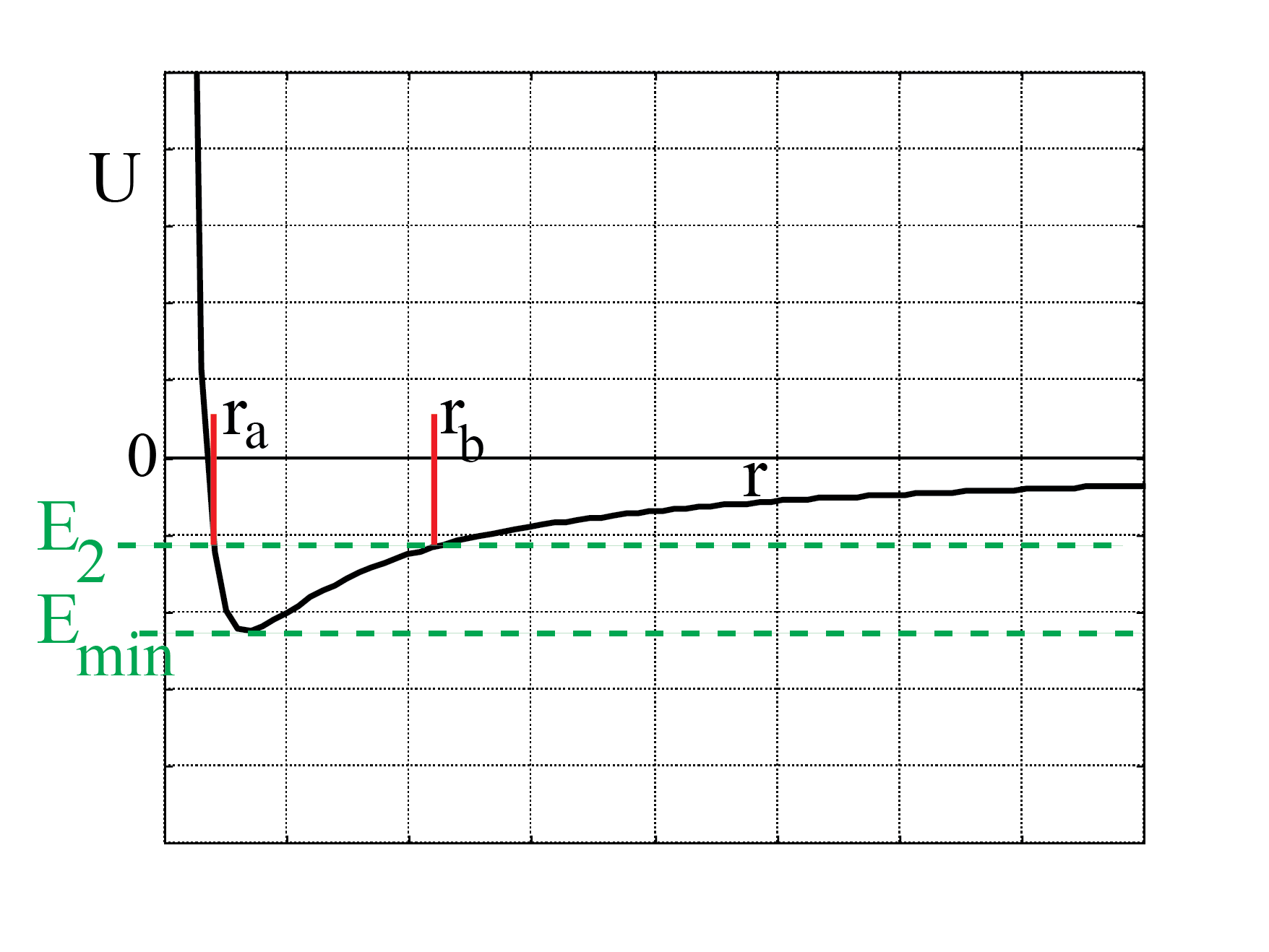
Figure 24:Total energy between 0 and minimum of effective potential.
Thus, the trajectory is confined between and . At both these end points, the planet will have zero radial velocity: . However, as before, the planet will still have angular momentum and thus still have a non-zero velocity. The planet will travel in the -plane between and . How? We don’t know yet.
N.B. Do realize, that the velocity is for this case not a constant. We already have established that it is linked to the angular momentum (which is a constant) and the distance to the origin.
Thus, if the planet is closer to it moves faster than close to . But it can not escape from .
Finally, we take the case that the total energy of the planet is positive, say a value of in Figure 25. Now we see that the planet can approach the sun, but not closer than a distance . The planet is attracted to the sun, but after reaching the closest distance it will move away and eventually reach infinity. Again note: at , the planet does have a non-zero velocity.
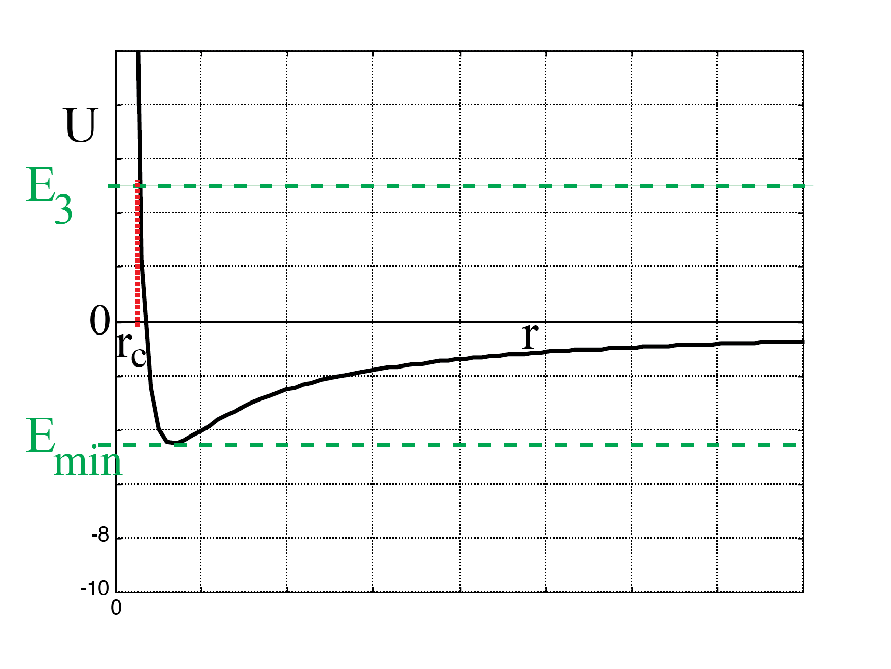
Figure 25:Total energy larger than 0.
4.6.3Ellipsoidal orbits
We are left with the task of showing that planets ‘circle’ the sun in an ellipse. From the above, we now know that this must mean that the total energy is smaller than zero: . We will not go over the details of the derivation, but leave that for another course.
The outcome of the analysis would be the following expression for the orbit in case of an ellipse:

Figure 26:Ellips in Cartesian coordinates.
This is an ellipse with semi major and minor-axis and , respectively. The center of the ellipse is located at . Note that the sun is in the origin and that seen from the center of the ellipse, the origin is at one of the focal points of the ellipse. Consequently, the orbit is not symmetric as viewed from the sun. We notice this on earth: the summer and winter (when the sun is closest respectively furthest from the sun) are not symmetric, even if we take the tilted axis of the earth into account.
The half and short long axis are given by:
with
and
This type of curve is know as the conic sections. That is, they can be found by intersecting a cone with a plane. See the animation below, where a plane is at various positions and at various angles intesecting a cone.
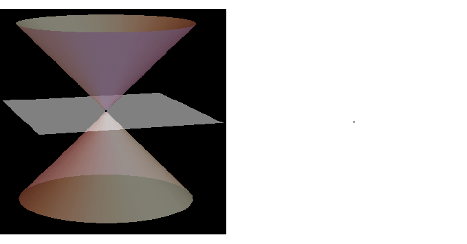
Figure 27:Conic sections animation created by Sara van der Werf, used with permission.
Note that in the definition of , the total energy of the system plays a role. This energy can be negative (see Figure 23). The minimum value of the effective potential energy is easily computed. It is and is realized when the planet is at a distance . For this case we have and the planet is moving in a circle around the sun, as we already argued above.
For the orbit is an ellipse as Kepler already had postulated (for these values of the orbit is a closed one).
For , the orbit is a parabola: the object will eventually move to infinity where it has exactly zero radial velocity.
Finally, for the trajectory is a hyperbola with the planet again moving to infinity.
Conclusion: according to Newton’s laws of mechanics, combined with the Gravitation force proposed by Newton, planets must move in ellipses around their star.
This holds for our solar system, but for any other star with planets as well. Research has shown that there are hundreds of solar systems out in the universe with thousands of planets moving around their star. See e.g. https://
4.6.4Kepler 3
We are left with proving Kepler’s third law:
Now that we know the orbit, this is not difficult. We concentrate on the motion during one lapse (one ‘year’). From Keppler’s 1 law we know that the area a planet sweeps out of its ellipse is given by
where is an integration constant. Furthermore, this way of writing makes that the area swept keeps increasing: after one round along the ellipse, we simply keep counting.
However, we can easily back out what happens after exactly one round, or one ‘year’. The total area swept is then, of course, the area of the ellipse itself, that is: in one year (time ) the area swept is . Hence we conclude:
If we put back what we found for and , we get
Thus, indeed Kepler was right. Moreover, we note that the constant is only depending on the mass of the sun. The same law will hold for other solar systems, but with a different constant.
In Figure 28 Kepler’s third law is shown for our solar system. The red data points are based on the measured ‘year’ of each planet and the distance to the sun. The blue line is the prediction from Newton’s theory.

Figure 28:Kepler 3 for our solar system.
4.7Speed of the planets & dark matter
Starting from Kepler 3, we can compute the orbital speed of a planet around the sun
Indeed if we measure the speed of the planets in the solar system this prediction holds, the velocity drops with the distance from the sun as (see figure). As we use the mass of the sun here.

Figure 30:From LibreTexts Physics, licensed under CC BY-NC-SA 4.0.
The distance is measured in Astronomical Units [AU], the distance from the earth to the sun (about 8.3 light minutes). Note that the earth is moving with an unbelievable 30 km/s, that is 105 km/h! Do you notice any of that? We will use this motion later with the Michelson-Morley experiment.
If we plot the same speed versus distance curve not for the planets in our solar system, but for stars orbiting the center of our galaxy, the milky way, then the picture looks very different. The far away stars orbit at a much higher speed than expected and the form of the found curve does not match .

Figure 31:Adapted from Wikimedia Commons, licensed under CC-SA 3.0.
This mismatch is not understood to this day! The mass here is calculated from the visible stars and the supermassive black holes at the center of the galaxy. But even if the mass is calculated wrongly, the shape of the dependency does not match. It turns out, this mismatch is observed in all galaxies! Apparently the law of gravity does not hold for large distances or there must be extra mass that increases the speed that we do not see. This mismatch has lead to the postulation of dark matter and an alternative formulation for the laws of gravity. This is the most disturbing problem in physics today; second is probably the interpretation of measurement in quantum mechanics (collapse of the wave function/Kopenhagen interpretation of Quantum Mechanics; multiverse theories).
The majority of all matter in the universe is believed to be dark. And we have no clue what it could be! Most scientist even think it must be non-baryonic, that is, other stuff than our well-known protons or neutrons. It remains most confusing.
The usual distance unit for distances in astronomy outside the solar system is not light years (ly), but parsec [pc], or kpc, or Mpc. One parsec is about 3.3 ly (or 1013 km). Note: stars visible to the eye are typically not more than a few hundred parsec away. The Milky Way is perfectly visible to the naked eye as a band/stripe of “milk” sprayed over the night sky. But you cannot see it anywhere close to Delft, there is much too much light from cities and greenhouses. Go to Scandinavia in the winter (“wintergatan”) or any place remote where there are few people. The reason you see a “band” in the night sky, is that the Milky Way is a spiral galaxy, sort of pancake shaped, and you see the band in the direction of the pancake.