2Newton’s Laws

2.1Newton’s Three Laws¶

Much of physics, in particular Classical Mechanics, rests on three laws that carry Newton’s name:

N1 has, in fact, been formulated by Galileo Galilei. Newton has, in his N2, build upon it: N1 is included in N2, after all:
if $\vec{F} = 0$, then $\frac{d\vec{p}}{dt} = 0 \rightarrow \vec{p} = \text{constant} \rightarrow \vec{v} = \text{constant}$, provided $m$ is a constant.

Most people know N2 as

For particles of constant mass, the two are equivalent:
if $m = \text{constant}$, then

Nevertheless, in many cases using the momentum representation is beneficial. The reason is that momentum is one of the key quantities in physics. This is due to the underlying conservation law, that we will derive in a minute. Moreover, using momentum allows for a new interpretation of force: force is that quantity that - provided it is allowed to act for some time interval on an object - changes the momentum of that object. This can be formally written as:

The latter quantity $\vec{I} \equiv \int \vec{F} dt$ is called the impulse.

In Newton’s Laws, velocity, acceleration and momentum are key quantities. We repeat here their formal definition.

Solution to Exercise 1

Interpret

Develop

First we make a sketch.

This is obviously a 1-dimensional problem. So, we can leave out the vector character of e.g. the force.

We will use $dp = F dt$:

$$dp = Fdt \Rightarrow \Delta p = \int_0^{\Delta t} Fdt = F \Delta t \rightarrow$$

(7)

$$p ( \Delta t) = p(0) + F \Delta t = mv_0 + F \Delta t \rightarrow$$

(8)

$$v ( \Delta t ) = v_0 + \frac{F}{m} \Delta t$$

(9)

Note that this example could also be solved by N2 in the form of $F = ma$. It is merely a matter of taste.

2.2Newton’s laws applied¶

2.2.1Force addition, subtraction and decomposition¶

Newton’s laws describe how forces affect motion, and applying them often requires combining multiple forces acting on an object, see Figure 3. This is done through vector addition, subtraction, and decomposition—allowing us to find the net force and analyze its components in different directions, see this chapter in the book on linear algebra for a full elaboration on vector addition and subtraction.

2.2.2Acceleration due to gravity¶

In most cases the forces acting on an object are not constant. However, there is a classical case that is treated in physics (already at secondary school level) where only one, constant force acts and other forces are neglected. Hence, according to Newton’s second law, the acceleration is constant.

When we first consider only the motion in the z-direction, we can derive:

Hence, for the velocity:

assuming $t_0=0 \text{ and } t_e=t \Rightarrow v(t)=v_0+at$ the position is described by

Rearranging:

Solution to Exercise 5

Interpret

Develop

Evaluate

Assess

Only gravity acts on the stone (in the downward direction). We will call the position of the stone at time $t$: $s(t)$
Initial conditions: $t=0 \rightarrow s(0) = s_0 = 1.5\mathrm{ m} \text{ and } \dot{s} = v = v_0 = 10 \mathrm{ m/s}$

1. $s(t) = \frac{1}{2}at^2 + v_0t + s_0$ Highest point reached when $\dot{s}=0$
2. $\Delta t = \frac{\Delta v}{a}$
3. $s(t) = \frac{1}{2}at^2 + v_0t + s_0$. We are interested in the stone hitting the ground. Thus, solve for $s(t)=0$ to find at what time this happens.

1. $\dot{s} = \vec{a}t + \vec{v}_0 = -gt + v_0 = 0 \Rightarrow t = 1.02 \text{s}$
   $s(1.02) = -\frac{1}{2}*9.81*1.02^2 + 10*1.02 + 1.5 = 6.6 \text{m}$
2. See above.
3. $\vec{s}(t) = \frac{1}{2}\vec{a}t^2 + \vec{v}_0t + \vec{s}_0 = \vec{s}_e$
   $t = \frac{-v_0\pm\sqrt{v_0^2-4(\frac{1}{2}a(s_0-s_e))}}{2\frac{1}{2}a} = \frac{-10\pm\sqrt{10^2-4(\frac{1}{2}(-9.81)(1.5))}}{-9.81}=2.18\text{s}$
   $v(2.18)=\dot{s}(2.18)=\vec{v}_0+\vec{a}t=10-9.81*2.18=-11.3 \text{m/s}$
   Note that $t=-0.14\text{s}$ is another solution, but not physically realistic.

The times we calculated are in the right order: First stone is tossed (at $t_0=0$), then it reaches its highest point (at $t_m=1.02 \mathrm{s}$). After that it falls and hits the ground at $t_e=2.18 \mathrm{s}$. Thus $t_0 \lt t_m \lt t_e$.

Furthermore, the velocity upon impact with the earth is negative as it should: the stone is falling downward. Its magnitude is on the order of the initial upward velocity, which makes sense. Finally, our answers have the right units.

NOTE: Some of these solutions can be derived more easily using the concept of conservation of energy which will be covered in one of the next chapters.

Solution to Exercise 7

The horizontal traveled distance is the same per time unit. For the vertical traveled distance it decreases until $v_y=0$ and then increases.

Interpret

Develop

Evaluate

The basic formulas are:

$$s_x(t)=v_xt$$

(22)

and

$$s_y(t)=v_yt-1/2gt^2$$

(23)

The horizontal traveled distance is given by:

$$s_x(t)=v_xt=v_0\cos(\theta)t$$

(24)

The time the object stays in the air is

$$s_y(t)=v_yt-1/2gt^2=0 \Rightarrow t=0 \text{ \& } t=\frac{2v_y}{g}=\frac{2v_0\sin(\theta)}{g}$$

(25)

Hence, the maximum distance traveled is:

$$s_x(t)=v_xt=v_0\cos(\theta)\frac{2v_0\sin(\theta)}{g}=\frac{2v_o^2\sin(\theta)\cos(\theta)}{g}$$

(26)

Note that the distance traveled is independent of the mass!

2.2.3Frictional forces¶

There are two main types of frictional force:

• Static friction prevents an object from starting to move. It adjusts in magnitude up to a maximum value, depending on how much force is trying to move the object. This maximum is given by

where $\mu_s$ is the coefficient of static friction and $N$ is the normal force. If the applied force exceeds this maximum, the object begins to slide.

• Kinetic (dynamic) friction opposes motion once the object is sliding. Its magnitude is generally constant and given by

where $\mu_k$ is the coefficient of kinetic friction. This force does not depend on the velocity of the object, only on the normal force and surface characteristics.

Friction always acts opposite to the direction of intended or actual motion and is essential in both preventing and controlling movement.

Values are approximate and can vary depending on surface conditions.

2.3Conservation of Momentum¶

From Newton’s 2$^{\text{nd}}$ and 3$^\text{rd}$ law we can easily derive the law of conservation of momentum.
Assume there are only two point-particle (i.e. particles with no size but with mass), that exert a force on each other. No other forces are present. From N2 we have:

From N3 we know:

And, thus by adding the two momentum equations we get:

Note the importance of the last conclusion: if objects interact via a mutual force then the total momentum of the objects can not change. No matter what the interaction is. It is easily extended to more interacting particles. The crux is that particles interact with one another via forces that obey N3. Thus for three interacting point particles we would have (with $\vec{F}_{ij}$ the force from particle i felt by particle j):

Sum these three equations:

For a system of $N$ particles, extension is straight forward.

2.3.1Momentum example¶

The above theoretical concept is simple in its ideas:

• a particle changes its momentum whenever a force acts on it;
• momentum is conserved;
• action = - reaction.

But it is incredible powerful and so generic, that finding when and how to use it is much less straight forward. The beauty of physics is its relatively small set of fundamental laws. The difficulty of physics is these laws can be applied to almost anything. The trick is how to do that, how to start and get the machinery running. That can be very hard. Luckily there is a recipe to master it: it is called practice.

Solution to Exercise 12

Let’s do this one together. We follow the standard approach of IDEA: Interpret (and make your sketch!), develop (think ‘model’), evaluate (solve your model) and assess (does it make any sense?).

Interpret

Develop

Evaluate

Assess

First a sketch: draw what is needed, no more, no less.

Actually this is half of the work, as when deciding what is needed we need to think what the problem really is. Above, is a sketch that could work. Both the object $m$ and the earth (mass $M$) are drawn schematically. On each of them acts a force, where we know that on $m$ standard gravity works. As a consequence of N3, a force equal in strength but opposite in direction acts on $M$.
Why do we draw forces? Well, the question mentions ‘momentum the particle hits the ground’. Momentum and forces are coupled via N2.

We have drawn a z-coordinate: might be handy to remind us that this looks like a 1D problem (remember: momentum and force are both vectors).

As a first step, we ignore the motion of the earth. Argument? The magnitude of the ratio of the acceleration of earth over object is given by:

$$\frac{a_e}{a_o} = \frac{| F_{o \rightarrow e} |/m_e}{| F_{e \rightarrow o} |/m_o} = \frac{m_o}{m_e}$$

(48)

here for the second equality we used N3.

For all practical purposes, the mass of the object is many orders of magnitude smaller than that of the earth. Hence, we can conclude that the acceleration of the earth is many orders of magnitude less than that of the object. The latter is of the order of $g$, gravity’s acceleration constant at the earth. Thus, the acceleration of the earth is next to zero and we can safely assume our lab system, that is connected to the earth, can be treated as an inertial system with, for us, zero velocity.

The remainder is straightforward. Now we have an object, that moves under a constant force. So its velocity will increase linearly in time:

$$\frac{dp}{dt} = -mg \Rightarrow p(t) = m\underbrace{v_0}_{=0} - mgt = -mgt$$

(49)

From the momentum we can calculate the velocity and from the velocity the position:

$$v = -gt \Rightarrow \frac{dz}{dt} = -gt \Rightarrow z(t) = \underbrace{z_0}_{=H} - \frac{1}{2}gt^2 = H - \frac{1}{2}gt^2$$

(50)

Solve for $z(T) = 0$ and find $T = \sqrt{\frac{2H}{g}}$. Substitute this into the relation for $v$: $v(T) = -\sqrt{2gH}$. As the earth-object system has conserved momentum, the velocity of the earth is to a good approximation:

$$p_e + p_o = 0 \Rightarrow v_e = - \frac{m_o}{m_e} v_o = \frac{m_o}{m_e} \sqrt{2gH}$$

(51)

We found that the particle changed its momentum from $p_i=0$ to $p_f=-mv$. The earth compensates for this, to keep momentum conserved. That gave that earth got a tiny, tiny upwards velocity. We could estimate the displacement of the earth. Suppose, the particle has mass $m$=1kg and is dropped from a height $H$=100m. Then we get for the velocity of the mass upon impact: $v=-44.3$m/s and a falling time $\Delta t$=4.5s. For the earth we thus find that during the process the velocity is smaller than $v_e$ and thus, the distance traveled by earth towards the mass is less than $\Delta x_e \lt v_e \Delta t = 1.6 \cdot 10^{-24}\mathrm{m}$. Indeed completely negligible, the size of the nucleus of an atom is many orders of magnitude bigger!

2.4Forces & Inertia¶

Newton’s laws introduce the concept of force. Forces have distinct features:

• forces are vectors, that is, they have magnitude and direction;
• forces change the motion of an object:
  • they change the velocity, i.e. they accelerate the object

• or, equally true, they change the momentum of an object

Many physicists like the second bullet: forces change the momentum of an object, but for that they need time to act.

Momentum is a more fundamental concept in physics than acceleration. That is another reason why physicists prefer the second way of looking at forces.

2.4.1Inertia¶

Inertia is denoted by the letter $m$ for mass. And mass is that property of an object that characterizes its resistance to changing its velocity. Actually, we should have written something like $m_i$, with subscript i denoting inertia.

Why? There is another property of objects, also called mass, that is part of Newton’s Gravitational Law.

Two bodies of mass $m_1$ and $m_2$ that are separated by a distance $r_{12}$ attract each other via the so-called gravitational force ($\hat{r}_{12}$ is a unit vector along the line connecting $m_1$ and $m_2$):

Here, we should have used a different symbol, rather than $m$. Something like $m_g$, as it is by no means obvious that the two ‘masses’ $m_i$ and $m_g$ refer to the same property. If you find that confusing, think about inertia and electric forces. Two particles with each an electric charge, $q_1$ and $q_2$, respectively exert a force on each other known as the Coulomb force:

We denote the property associated with electric forces by $q$ and call it charge. We have no problem writing

We do not confuse $q$ by $m$ or vice versa. They are really different quantities: $q$ tells us that the particle has a property we call ‘charge’ and that it will respond to other charges, either being attracted to, or repelled from. How fast it will respond to this force of another charged particle depends on $m$. If $m$ is big, the particle will only get a small acceleration; the strength of the force does not depend on $m$ at all. So far, so good. But what about $m_g$? That property of a particle that makes it being attracted to another particle with this same property, that we could have called ‘gravitational charge’. It is clearly different from ‘electrical charge’. But would it have been logical that it was also different from the property inertial mass, $m_i$?

As far as we can tell (via experiments) $m_i$ and $m_g$ are the same. Actually, it was Einstein who postulated that the two are referring to the same property of an object: there is no difference.

2.4.1.1Force field¶

We have seen, forces like gravity and electrostatics act between objects. When you push a car, the force is applied locally, through direct contact. In contrast, gravitational and electrostatic forces act over a distance — they are present throughout space, though they still depend on the positions of the objects involved.

One powerful way to describe how a force acts at different locations in space is through the concept of a force field. A force field assigns a force vector (indicating both direction and magnitude) to every point in space, telling you what force an object would experience if placed there.

For example, the graph below at the left shows a gravitational field, described by $\vec{F}_g=G\frac{mM}{r^2}\hat{r}$. Any object entering this field is attracted toward the central mass with a force that depends on its distance from that mass’s center.

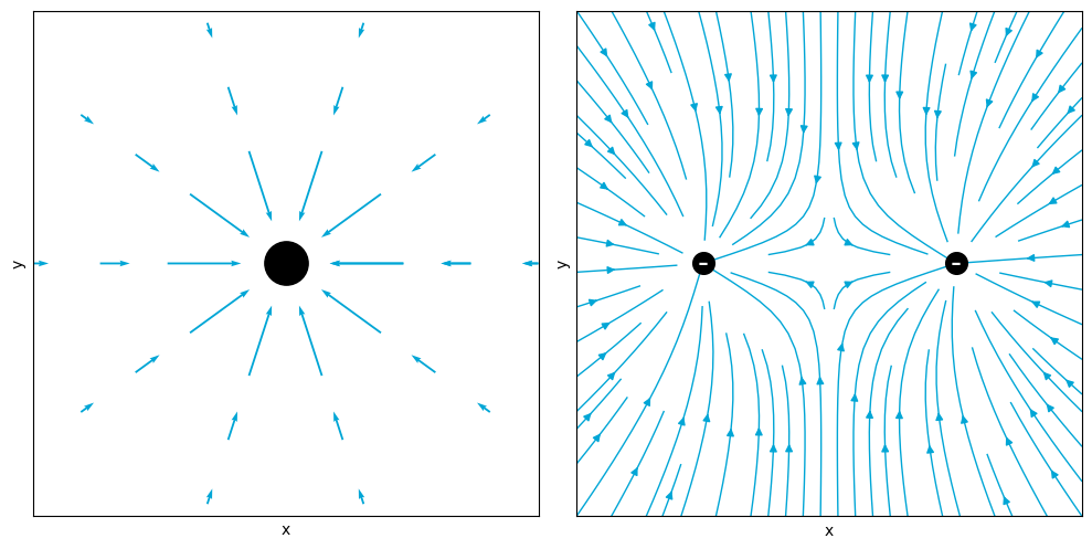
2.4.1.2Measuring mass or force¶

So far we did not address how to measure force. Neither did we discuss how to measure mass. This is less trivial than it looks at first side. Obviously, force and mass are coupled via N2: $F = m a$.

The acceleration can be measured when we have a ruler and a clock, i.e. once we have established how to measure distance and how to measure time intervals, we can measure position as a function of time and from that velocity and acceleration.

But how to find mass? We could agree upon a unit mass, an object that represents by definition 1kg. In fact we did. But that is only step one. The next question is: how do we compare an unknown mass to our standard. A first reaction might be: put them on a balance and see how many standard kilograms you need (including fractions of it) to balance the unknown mass. Sounds like a good idea, but is it? Unfortunately, the answer is not a ‘yes’.

As on second thought: the balance compares the pull of gravity. Hence, it ‘measures’ gravitational mass, rather than inertia. Luckily, Newton’s laws help. Suppose we let two objects, our standard mass and the unknown one, interact under their mutual interaction force. Every other force is excluded. Then, on account on N2 we have

where we used N3 for the last equality. Clearly, if we take the ratio of these two equations we get:

irrespective of the strength or nature of the forces involved. We can measure acceleration and thus with this rule express the unknown mass in terms of our standard.

Now that we know how to determine mass, we also have solved the problem of measuring force. We just measure the mass and the acceleration of an object and from N2 we can find the force. This allows us to develop ‘force measuring equipment’ that we can calibrate using the method discussed above.

2.4.2Eötvös experiment on mass¶

The question whether inertial mass and gravitational mass are the same has put experimentalists to work. It is by no means an easy question. Gravity is a very weak force. Moreover, determining that two properties are identical via an experiment is virtually impossible due to experimental uncertainty. Experimentalist can only tell the outcome is ‘identical’ within a margin. Newton already tried to establish experimentally that the two forms of mass are the same. However, in his days the inaccuracy of experiments was rather large. Dutch scientist Simon Stevin concluded in 1585 that the difference must be less than 5%. He used his famous ‘drop masses from the church’ experiments for this (they were primarily done to show that every mass falls with the same acceleration).

A couple of years later, Galilei used both fall experiments and pendula to improve this to: less than 2%. In 1686, Newton using pendula managed to bring it down to less than 1‰ .

An important step forward was set by the Hungarian physicist, Loránd Eötvös (1848-1918). We will here briefly introduce the experiment. For a full analysis, we need knowledge about angular momentum and centrifugal forces that we do not deal with in this book.

2.4.2.1The experiment¶

The essence of the Eötvös experiment is finding a set up in which both gravity (sensitive to the gravitational mass) and some inertial force (sensitive to the inertial mass) are present. Obviously, gravitational forces between two objects out of our daily life are extremely small. This will be very difficult to detect and thus introduce a large error if the experiment relies on measuring them. Eötvös came up with a different idea. He connected two different objects with different masses, $m_1$ and $m_2$, via a (almost) massless rod. Then, he attached a thin wire to the rod and let it hang down.

This is a sensitive device: any mismatch in forces or torques will have the setup either tilt or rotate a bit. Eötvös attached a tiny mirror to one of the arms of the rod. If you shine a light beam on the mirror and let it reflect and be projected on a wall, then the smallest deviation in position will be amplified to create a large motion of the light spot on the wall.

In Eötvös experiment two forces are acting on each of the masses: gravity, proportional to $m_g$, but also the centrifugal force $F_c = m_i R \omega^2$, the centrifugal force stemming from the fact that the experiment is done in a frame of reference rotating with the earth. This force is proportional to the inertial mass. The experiment is designed such that if the rod does not show any rotation around the vertical axis, then the gravitational mass and inertial mass must be equal. It can be done with great precision and Eötvös observed no measurable rotation of the rod. From this he could conclude that the ratio of the gravitational over inertial mass differed less from 1 than $5 \cdot 10^{-8}$. Currently, experimentalist have brought this down to $1 \cdot 10^{-15}$.